7.2 Linked Genes Segregate Together While Crossing Over Produces Recombination Between Them
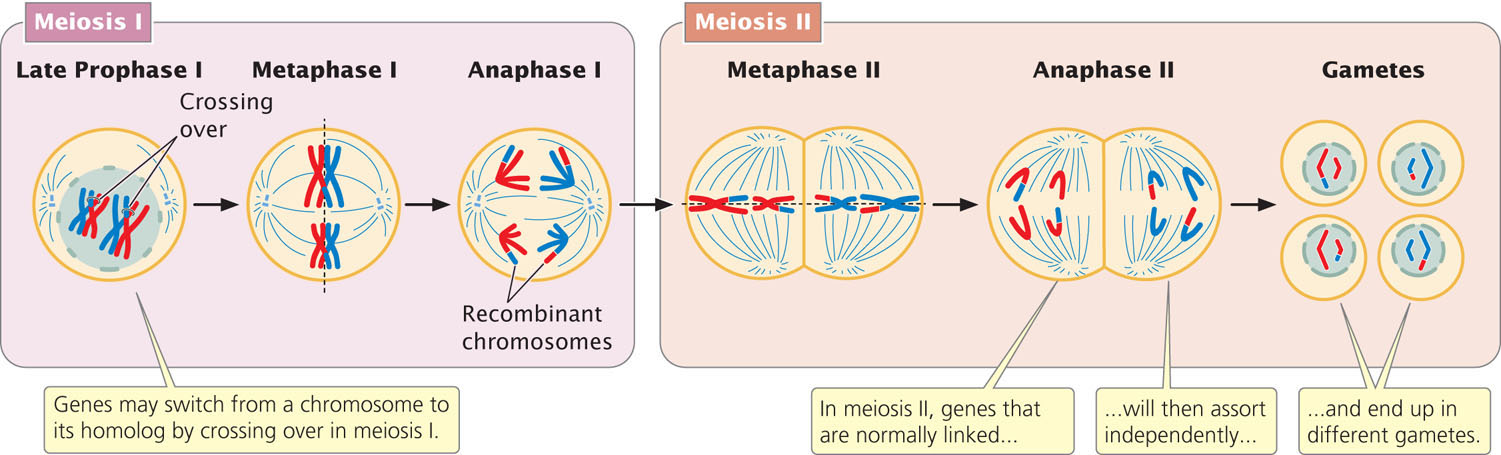
Genes that are close together on the same chromosome usually segregate as a unit and are therefore inherited together. However, genes occasionally switch from one homologous chromosome to the other through the process of crossing over (see Chapter 2), as illustrated in Figure 7.3. Crossing over results in recombination; it breaks up the associations of genes that are close together on the same chromosome. Linkage and crossing over can be seen as processes that have opposite effects: linkage keeps particular genes together, and crossing over mixes them up, producing new combinations of genes. In Chapter 5, we considered a number of exceptions and extensions to Mendel’s principles of heredity. The concept of linked genes adds a further complication to interpretations of the results of genetic crosses. However, with an understanding of how linkage affects heredity, we can analyze crosses for linked genes and successfully predict the types of progeny that will be produced.
168
Notation for Crosses with Linkage
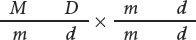
In analyzing crosses with linked genes, we must know not only the genotypes of the individuals crossed, but also the arrangement of the genes on the chromosomes. To keep track of this arrangement, we introduce a new system of notation for presenting crosses with linked genes. Consider a cross between an individual homozygous for dominant alleles at two linked loci and another individual homozygous for recessive alleles at those loci (AA BB × aa bb). For linked genes, it’s necessary to write out the specific alleles as they are arranged on each of the homologous chromosomes:
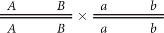
In this notation, each line represents one of the two homologous chromosomes. Inheriting one chromosome from each parent, the F1 progeny will have the following genotype:
Here, the importance of designating the alleles on each chromosome is clear. One chromosome has the two dominant alleles A and B, whereas the homologous chromosome has the two recessive alleles a and b. The notation can be simplified by drawing only a single line, with the understanding that genes located on the same side of the line lie on the same chromosome:

This notation can be simplified further by separating the alleles on each chromosome with a slash: AB/ab.
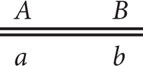
Remember that the two alleles at a locus are always located on different homologous chromosomes and therefore must lie on opposite sides of the line. Consequently, we would never write the genotypes as

because the alleles A and a can never be on the same chromosome. It is also important to always keep the same order of the genes on both sides of the line; thus, we should never write

because it would imply that alleles A and b are allelic (at the same locus).
Complete Linkage Compared with Independent Assortment
We will first consider what happens to genes that exhibit complete linkage, meaning that they are located very close together on the same chromosome and do not exhibit crossing over. Genes are rarely completely linked but, by assuming that no crossing over takes place, we can see the effect of linkage more clearly. We will then consider what happens when genes assort independently. Finally, we will consider the results obtained if the genes are linked but exhibit some crossing over.
A testcross reveals the effects of linkage. For example, if a heterozygous individual is test-crossed with a homozygous recessive individual (Aa Bb × aa bb), the alleles that are present in the gametes contributed by the heterozygous parent will be expressed in the phenotype of the offspring because the homozygous parent could not contribute dominant alleles that might mask them. Consequently, traits that appear in the progeny reveal which alleles were transmitted by the heterozygous parent.
169
Consider a pair of linked genes in tomato plants. One of the genes affects the type of leaf: an allele for mottled leaves (m) is recessive to an allele that produces normal leaves (M). Nearby on the same chromosome the other gene determines the height of the plant: an allele for dwarf (d) is recessive to an allele for tall (D).
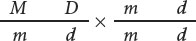
Testing for linkage can be done with a testcross, which requires a plant heterozygous for both characteristics. A geneticist might produce this heterozygous plant by crossing a variety of tomato that is homozygous for normal leaves and tall height with a variety that is homozygous for mottled leaves and dwarf height:
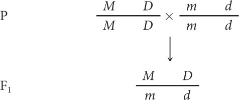
The geneticist would then use these F1 heterozygotes in a testcross, crossing them with plants homozygous for mottled leaves and dwarf height:
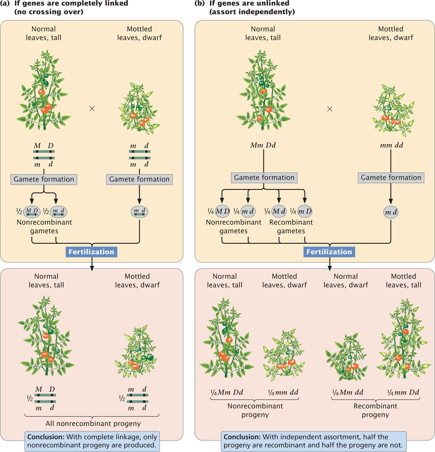
The results of this testcross are diagrammed in Figure 7.4a. The heterozygote produces two types of gametes: some with the M D chromosome and others with the m d chromosome. Because no crossing over takes place, these gametes are the only types produced by the heterozygote. Notice that these gametes contain only combinations of alleles that were present in the original parents: either the allele for normal leaves together with the allele for tall height (M and D) or the allele for mottled leaves together with the allele for dwarf height (m and d). Gametes that contain only original combinations of alleles present in the parents are nonrecombinant gametes, or parental gametes.
170
The homozygous parent in the testcross produces only one type of gamete; it contains chromosome m d and pairs with one of the two gametes generated by the heterozygous parent (see Figure 7.4a). Two types of progeny result: half have normal leaves and are tall:

and half have mottled leaves and are dwarf:

These progeny display the original combinations of traits present in the P generation and are nonrecombinant progeny, or parental progeny. No new combinations of the two traits, such as normal leaves with dwarf height or mottled leaves with tall height appear in the offspring, because the genes affecting the two traits are completely linked and are inherited together. New combinations of traits could arise only if the physical connection between M and D or between m and d were broken.
These results are distinctly different from the results that are expected when genes assort independently (Figure 7.4b). If the M and D loci assorted independently, the heterozygous plant (Mm Dd) would produce four types of gametes: two nonrecombinant gametes containing the original combinations of alleles (M D and m d) and two gametes containing new combinations of alleles (M d and m D). Gametes with new combinations of alleles are called recombinant gametes. With independent assortment, nonrecombinant and recombinant gametes are produced in equal proportions. These four types of gametes join with the single type of gamete produced by the homozygous parent of the testcross to produce four kinds of progeny in equal proportions (see Figure 7.4b). The progeny with new combinations of traits formed from recombinant gametes are termed recombinant progeny.
CONCEPTS
A testcross in which one of the plants is heterozygous for two completely linked genes yields two types of progeny, each type displaying one of the original combinations of traits present in the P generation. In contrast, independent assortment produces four types of progeny in a 1 : 1 : 1 : 1 ratio—two types of recombinant progeny and two types of nonrecombinant progeny in equal proportions.
Crossing Over with Linked Genes
Usually, there is some crossing over between genes that lie on the same chromosome, producing new combinations of traits. Genes that exhibit crossing over are incompletely linked. Let’s see how incomplete linkage affects the results of a cross.
Theory
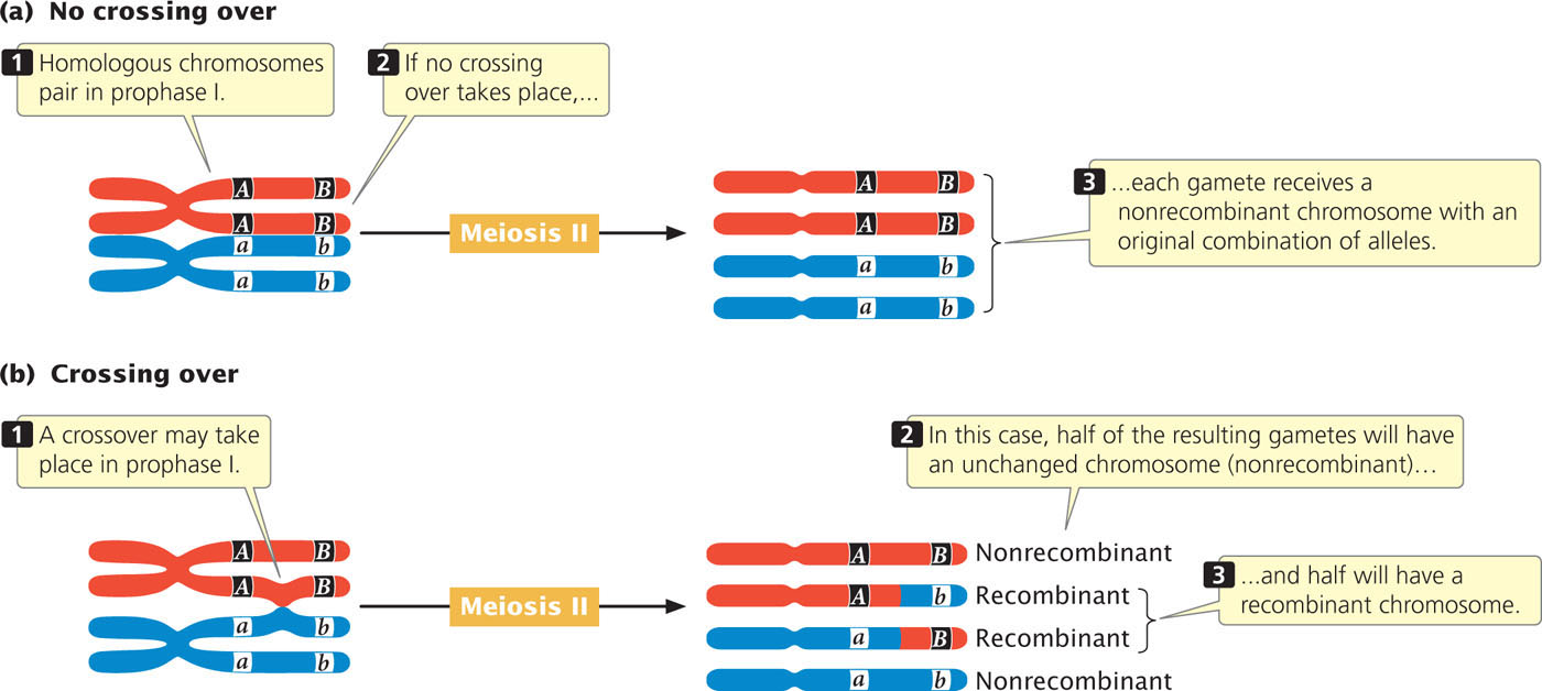
The effect of crossing over on the inheritance of two linked genes is shown in Figure 7.5. Crossing over, which takes place in prophase I of meiosis, is the exchange of genetic material between nonsister chromatids (see Figures 2.16 and 2.18). After a single crossover has taken place, the two chromatids that did not participate in crossing over are unchanged; gametes that receive these chromatids are nonrecombinants. The other two chromatids, which did participate in crossing over, now contain new combinations of alleles; gametes that receive these chromatids are recombinants. For each meiosis in which a single crossover takes place, two nonrecombinant gametes and two recombinant gametes will be produced. This result is the same as that produced by independent assortment (see Figure 7.4b); so, when crossing over between two loci takes place in every meiosis, it is impossible to determine whether the genes are on the same chromosome and crossing over took place or whether the genes are on different chromosomes.
171
For closely linked genes, crossing over does not take place in every meiosis. In meioses in which there is no crossing over, only nonrecombinant gametes are produced. In meioses in which there is a single crossover, half the gametes are recombinants and half are nonrecombinants (because a single crossover affects only two of the four chromatids. Because each crossover leads to half recombinant gametes and half nonrecombinant gametes, the total percentage of recombinant gametes is always half the percentage of meioses in which crossing over takes place. Even if crossing over between two genes takes place in every meiosis, only 50% of the resulting gametes will be recombinants. Thus, the frequency of recombinant gametes is always half the frequency of crossing over and the maximum proportion of recombinant gametes is 50%.
CONCEPTS
Linkage between genes causes them to be inherited together and reduces recombination; crossing over breaks up the associations of such genes. In a testcross for two linked genes, each crossover produces two recombinant gametes and two nonrecombinants. The frequency of recombinant gametes is half the frequency of crossing over, and the maximum frequency of recombinant gametes is 50%.
 CONCEPT CHECK 1
For single crossovers, the frequency of recombinant gametes is half the frequency of crossing over because
- a testcross between a homozygote and heterozygote produces
 heterozygous and
homozygous progeny.
heterozygous and
homozygous progeny. - the frequency of recombination is always 50%.
- each crossover takes place between only two of the four chromatids of a homologous pair.
- crossovers take place in about 50% of meioses.
Application
Let’s apply what we have learned about linkage and recombination to a cross between tomato plants that differ in the genes that encode leaf type and plant height. Assume now that these genes are linked and that some crossing over takes place between them. Suppose a geneticist carried out the testcross described earlier:
When crossing over takes place in the genes for leaf type and height, two of the four gametes produced are recombinants. When there is no crossing over, all four resulting gametes are nonrecombinants. Because each crossover produces half recombinant gametes and half nonrecombinant gametes, the majority of gametes will be nonrecombinants (Figure 7.6a). These gametes then unite with gametes produced by the homozygous recessive parent, which contain only the recessive alleles, resulting in mostly nonrecombinant progeny and a few recombinant progeny (Figure 7.6b). In this cross, we see that 55 of the testcross progeny have normal leaves and are tall and that 53 have mottled leaves and are dwarf. These plants are the nonrecombinant progeny, containing the original combinations of traits that were present in the parents. Of the 123 progeny, 15 have new combinations of traits that were not seen in the parents: 8 have normal leaves and are dwarf, and 7 have mottled leaves and are tall. These plants are the recombinant progeny.
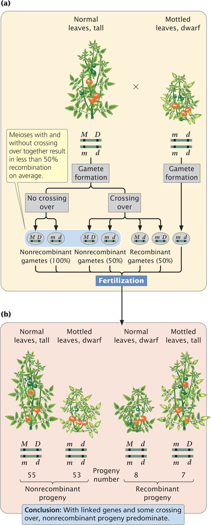
The results of a cross such as the one illustrated in Figure 7.6 reveal several things. A testcross for two independently assorting genes is expected to produce a 1 : 1 : 1 : 1 phenotypic ratio in the progeny. The progeny of this cross clearly do not exhibit such a ratio so we might suspect that the genes are not assorting independently. When linked genes undergo some crossing over, the result is mostly nonrecombinant progeny and fewer recombinant progeny. This result is what we observe among the progeny of the testcross illustrated in Figure 7.6, so we conclude that the two genes show evidence of linkage with some crossing over.
Calculating Recombination Frequency
The percentage of recombinant progeny produced in a cross is called the recombination frequency, which is calculated as follows:
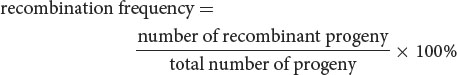
In the testcross shown in Figure 7.6, 15 progeny exhibit new combinations of traits, so the recombination frequency is:

Thus, 12.2% of the progeny exhibit new combinations of traits resulting from crossing over. The recombination frequency can also be expressed as a decimal fraction (0.122). ![]() TRY PROBLEM 15
TRY PROBLEM 15
172
Coupling and Repulsion
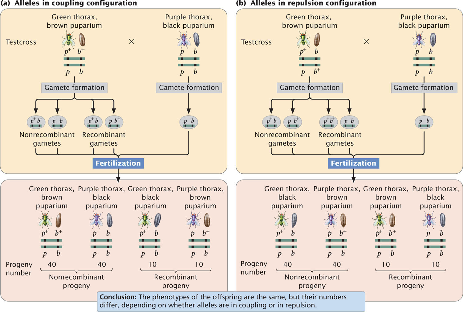
In crosses for linked genes, the arrangement of alleles on the homologous chromosomes is critical in determining the outcome of the cross. For example, consider the inheritance of two genes in the Australian blowfly, Lucilia cuprina. In this species, one locus determines the color of the thorax: a purple thorax (p) is recessive to the normal green thorax (p+). A second locus determines the color of the puparium: a black puparium (b) is recessive to the normal brown puparium (b+). The loci for thorax color and puparium color are located close together on the chromosome. Suppose that we test-cross a fly that is heterozygous at both loci with a fly that is homozygous recessive at both. Because these genes are linked, there are two possible arrangements on the chromosomes of the heterozygous progeny fly. The dominant alleles for green thorax (p+) and brown puparium (b+) might reside on one chromosome of the homologous pair, and the recessive alleles for purple thorax (p) and black puparium (b) might reside on the other homologous chromosome:

This arrangement, in which wild-type alleles are found on one chromosome and mutant alleles are found on the other chromosome, is referred to as the coupling, or cis configuration. Alternatively, one chromosome might carry the alleles for green thorax (p+) and black puparium (b), and the other chromosome might carry the alleles for purple thorax (p) and brown puparium (b+):

This arrangement, in which each chromosome contains one wild-type and one mutant allele, is called the repulsion, or trans configuration. Whether the alleles in the heterozygous parent are in coupling or repulsion determines which phenotypes will be most common among the progeny of a testcross.
When the alleles are in the coupling configuration, the most numerous progeny types are those with a green thorax and brown puparium and those with a purple thorax and black puparium (Figure 7.7a). However, when the alleles of the heterozygous parent are in repulsion, the most numerous progeny types are those with a green thorax and black puparium and those with a purple thorax and brown puparium (Figure 7.7b). Notice that the genotypes of the parents in Figure 7.7a and b are the same (p+ p b+ b × pp bb) and that the dramatic difference in the phenotypic ratios of the progeny in the two crosses results entirely from the configuration—coupling or repulsion—of the chromosomes. Knowledge of the arrangement of the alleles on the chromosomes is essential to accurately predict the outcome of crosses in which genes are linked.
173
CONCEPTS
In a cross, the arrangement of linked alleles on the chromosomes is critical for determining the outcome. When two wild-type alleles are on one homologous chromosome and two mutant alleles are on the other, they are in the coupling configuration; when each chromosome contains one wild-type allele and one mutant allele, the alleles are in repulsion.
CONCEPT CHECK 2
The following testcross produces the progeny shown: Aa Bb × aa bb → 10 Aa Bb, 40 Aa bb, 40 aa Bb, 10 aa bb. Were the A and B alleles in the Aa Bb parent in coupling or in repulsion?
CONNECTING CONCEPTS: Relating Independent Assortment, Linkage, and Crossing Over
We have now considered three situations concerning genes at different loci. First, the genes may be located on different chromosomes; in this case, they exhibit independent assortment and combine randomly when gametes are formed. An individual heterozygous at two loci (Aa Bb) produces four types of gametes (A B, a b, A b, and a B) in equal proportions: two types of nonrecombinants and two types of recombinants. In a testcross, these gametes will result in four types of progeny in equal proportions (Table 7.1).
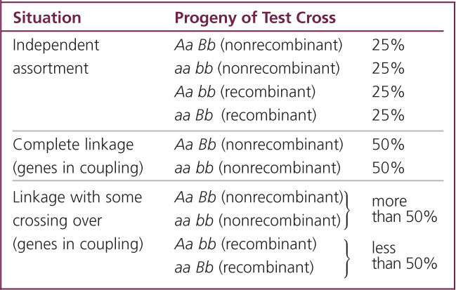
Second, the genes may be completely linked—meaning that they are on the same chromosome and lie so close together that crossing over between them is rare. In this case, the genes do not recombine. An individual heterozygous for two closely linked genes in the coupling configuration

produces only the nonrecombinant gametes containing alleles A B or a b; the alleles do not assort into new combinations such as A b or a B. In a testcross, completely linked genes will produce only two types of progeny, both nonrecombinants, in equal proportions (see Table 7.1).
The third situation, incomplete linkage, is intermediate between the two extremes of independent assortment and complete linkage. Here, the genes are physically linked on the same chromosome, which prevents independent assortment. However, occasional crossovers break up the linkage and allow the genes to recombine. With incomplete linkage, an individual heterozygous at two loci produces four types of gametes—two types of recombinants and two types of nonrecombinants—but the nonrecombinants are produced more frequently than the recombinants because crossing over does not take place in every meiosis. In the testcross, these gametes result in four types of progeny, with the nonrecombinants more frequent than the recombinant (see Table 7.1).
174
Earlier in the chapter, the term recombination was defined as the sorting of alleles into new combinations. We’ve now considered two types of recombination that differ in the mechanism that generates these new combinations of alleles. Interchromosomal recombination takes place between genes located on different chromosomes. It arises from independent assortment—the random segregation of chromosomes in anaphase I of meiosis—and is the kind of recombination that Mendel discovered while studying dihybrid crosses. A second type of recombination, intrachromosomal recombination, takes place between genes located on the same chromosome. This recombination arises from crossing over—the exchange of genetic material in prophase I of meiosis. Both types of recombination produce new allele combinations in the gametes so they cannot be distinguished by examining the types of gametes produced. Nevertheless, they can often be distinguished by the frequencies of types of gametes: interchromosomal recombination produces 50% nonrecombinant gametes and 50% recombinant gametes, whereas intrachromosomal recombination frequently produces more than 50% nonrecombinant gametes and less than 50% recombinant gametes. However, when the genes are very far apart on the same chromosome, crossing over takes place in every meiotic division, leading to 50% recombinant gametes and 50% nonrecombinant gametes. This result is the same as in independent assortment of genes located on different chromosomes (interchromosomal recombination). Thus, intrachromosomal recombination of genes that lie far apart on the same chromosome and interchromosomal recombination are phenotypically indistinguishable.
Evidence for the Physical Basis of Recombination
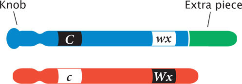
Walter Sutton’s chromosome theory of inheritance, which stated that genes are physically located on chromosomes, was supported by Nettie Stevens and Edmund Wilson’s discovery that sex was associated with a specific chromosome in insects (and Calvin Bridges’s demonstration that nondisjunction of X chromosomes was related to the inheritance of eye color in Drosophila (Chapter 4). Further evidence for the chromosome theory of heredity came in 1931, when Harriet Creighton and Barbara McClintock (Figure 7.8) obtained evidence that intrachromosomal recombination was the result of physical exchange between chromosomes. Creighton and McClintock discovered a strain of corn that had an abnormal chromosome 9, containing a densely staining knob at one end and a small piece of another chromosome attached to the other end. This aberrant chromosome allowed them to visually distinguish the two members of a homologous pair.
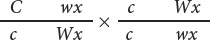
Creighton and McClintock studied the inheritance of two traits in corn determined by genes on chromosome 9. At one locus, a dominant allele (C) produced colored kernels, whereas a recessive allele (c) produced colorless kernels. At a second, linked locus, a dominant allele (Wx) produced starchy kernels, whereas a recessive allele (wx) produced waxy kernels. They obtained a plant that was heterozygous at both loci in repulsion, with the alleles for colored and waxy on the aberrant chromosome and the alleles for colorless and starchy on the normal chromosome:
175
They then crossed this heterozygous plant with one that was homozygous for colorless and heterozygous for waxy (with both chromosomes normal):
This cross will produce different combinations of traits in the progeny, but the only way that colorless and waxy progeny can arise is through crossing over in the doubly heterozygous parent:
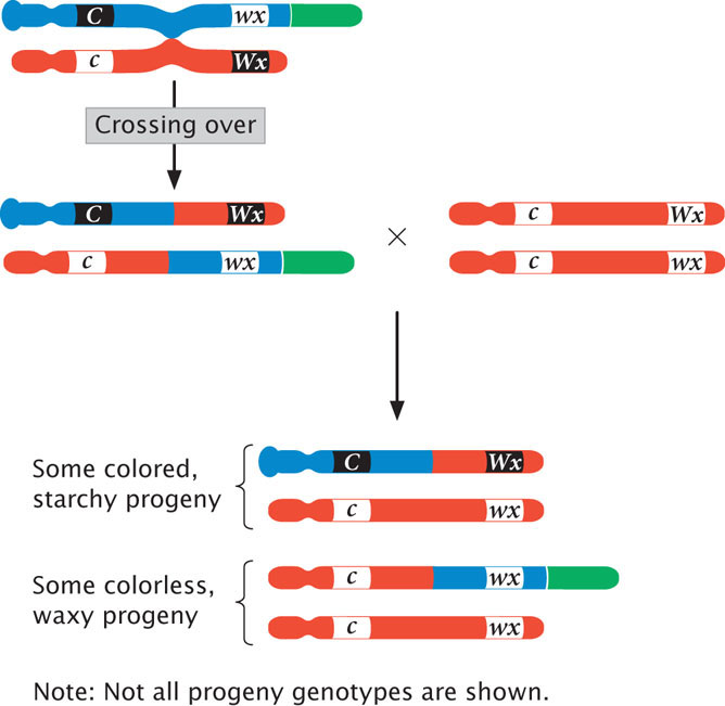
Notice that, if crossing over entails physical exchange between the chromosomes, then the colorless, waxy progeny resulting from recombination should have a chromosome with an extra piece but not a knob. Furthermore, some of the colored, starchy progeny should possess a knob but not the extra piece. This outcome is precisely what Creighton and McClintock observed, confirming the chromosomal theory of inheritance. Curt Stern provided a similar demonstration by using chromosomal markers in Drosophila at about the same time. We will examine the molecular basis of recombination in more detail in Chapter 12.
Predicting the Outcomes of Crosses with Linked Genes
Knowing the arrangement of alleles on a chromosome allows us to predict the types of progeny that will result from a cross entailing linked genes and to determine which of these types will be the most numerous. Determining the proportions of the types of offspring requires an additional piece of information—the recombination frequency. The recombination frequency provides us with information about how often the alleles in the gametes appear in new combinations, allowing us to predict the proportions of offspring phenotypes that will result from a specific cross with linked genes.
In cucumbers, smooth fruit (t) is recessive to warty fruit (T) and glossy fruit (d) is recessive to dull fruit (D). Geneticists have determined that these two genes exhibit a recombination frequency of 16%. Suppose that we cross a plant homozygous for warty and dull fruit with a plant homozygous for smooth and glossy fruit and then carry out a test-cross by using the F1:
What types and proportions of progeny will result from this testcross?
Four types of gametes will be produced by the heterozygous parent, as shown in Figure 7.9: two types of nonrecombinant gametes ( T D and t d ) and two types of recombinant gametes ( T d and t D ). The recombination frequency tells us that 16% of the gametes produced by the heterozygous parent will be recombinants. Because there are two types of recombinant gametes, each should arise with a frequency of 16%/2 = 8%. This frequency can also be represented as a probability of 0.08. All the other gametes will be nonrecombinants, so they should arise with a frequency of 100% − 16% = 84%. Because there are two types of nonrecombinant gametes, each should arise with a frequency of 84%/2 = 42% (or 0.42). The other parent in the testcross is homozygous and therefore produces only a single type of gamete ( t d ) with a frequency of 100% (or 1.00).
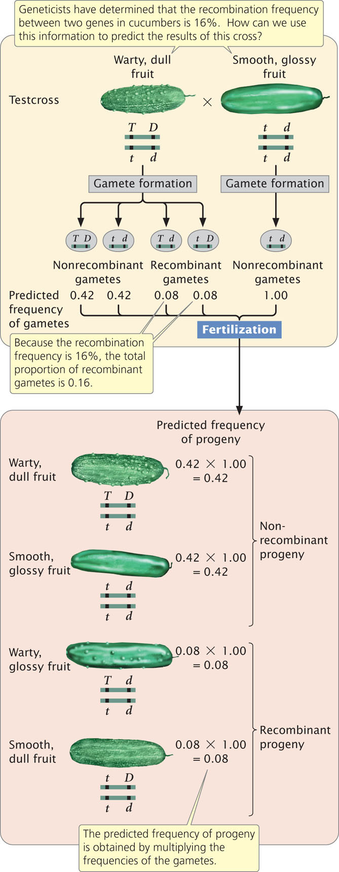
Four types of progeny result from the testcross (see Figure 7.9). The expected proportion of each type can be determined by using the multiplication rule (see Chapter 3), multiplying together the probability of each gamete. Testcross progeny with warty and dull fruit

appear with a frequency of 0.42 (the probability of inheriting a gamete with chromosome T D from the heterozygous parent) × 1.00 (the probability of inheriting a gamete with chromosome t d from the recessive parent) = 0.42. The proportions of the other types of F2 progeny can be calculated in a similar manner (see Figure 7.9). This method can be used for predicting the outcome of any cross with linked genes for which the recombination frequency is known.
176
Testing for Independent Assortment
In some crosses, the genes are obviously linked because there are clearly more nonrecombinant progeny than recombinant progeny. In other crosses, the difference between independent assortment and linkage isn’t as obvious. For example, suppose we did a testcross for two pairs of genes, such as Aa Bb × aa bb, and observed the following numbers of progeny: 54 Aa Bb, 56 aa bb, 42 Aa bb, and 48 aa Bb. Is this outcome the 1 : 1 : 1 : 1 ratio we would expect if A and B assorted independently? Not exactly, but it’s pretty close. Perhaps these genes assorted independently and chance produced the slight deviations between the observed numbers and the expected 1 : 1 : 1 : 1 ratio. Alternatively, the genes might be linked, with considerable crossing over taking place between them, and so the number of nonrecombinants is only slightly greater than the number of recombinants. How do we distinguish between the role of chance and the role of linkage in producing deviations from the results expected with independent assortment?
We encountered a similar problem in crosses in which genes were unlinked—the problem of distinguishing between deviations due to chance and those due to other factors. We addressed this problem (in Chapter 3) with the chi-square goodness-of-fit test, which helps us evaluate the likelihood that chance alone is responsible for deviations between the numbers of progeny that we observed and the numbers that we expected by applying the principles of inheritance. Here, we are interested in a different question: is the inheritance of alleles at one locus independent of the inheritance of alleles at a second locus? If the answer to this question is yes, then the genes are assorting independently; if the answer is no, then the genes are probably linked.
A possible way to test for independent assortment is to calculate the expected probability of each progeny type, assuming independent assortment, and then use the chi-square goodness-of-fit test to evaluate whether the observed numbers deviate significantly from the expected numbers. With independent assortment, we expect  of each phenotype:
Aa Bb,
aa bb,
Aa bb, and
aa Bb. This expected probability of each genotype is based on the multiplication rule of probability (see Chapter 3). For example, if the probability of Aa is
and the probability of Bb is
, then the probability of Aa Bb is
×
=
. In this calculation, we are making two assumptions: (1) the probability of each single-locus genotype is
, and (2) genotypes at the two loci are inherited independently (
×
=
).
of each phenotype:
Aa Bb,
aa bb,
Aa bb, and
aa Bb. This expected probability of each genotype is based on the multiplication rule of probability (see Chapter 3). For example, if the probability of Aa is
and the probability of Bb is
, then the probability of Aa Bb is
×
=
. In this calculation, we are making two assumptions: (1) the probability of each single-locus genotype is
, and (2) genotypes at the two loci are inherited independently (
×
=
).
One problem with this approach is that a significant chi-square value can result from a violation of either assumption. If the genes are linked, then the inheritance of genotypes at the two loci are not independent (assumption 2), and we will get a significant deviation between observed and expected numbers. But we can also get a significant deviation if the probability of each single-locus genotype is not
(assumption 1), even when the genotypes are assorting independently. We may obtain a significant deviation, for example, if individuals with one genotype have a lower probability of surviving or the penetrance of a genotype is not 100%. We could test both assumptions by conducting a series of chi-square tests, first testing the inheritance of genotypes at each locus separately (assumption 1) and then testing for independent assortment (assumption 2). However, a faster method is to test for independence in genotypes with a chi-square test of independence.
177
The Chi-Square Test of Independence
The chi-square test of independence allows us to evaluate whether the segregation of alleles at one locus is independent of the segregation of alleles at another locus, without making any assumption about the probability of single-locus genotypes. To illustrate this analysis, we will examine results from a cross between German cockroaches, in which yellow body (y) is recessive to brown body (y+) and curved wings (cv) are recessive to straight wings (cv+). A testcross (y+ y cv+cv × yy cvcv) produced the progeny shown in Figure 7.10a. If the segregation of alleles at each locus is independent, then the proportion of progeny with y+y and yy genotypes should be the same for cockroaches with genotype cv+cv and for cockroaches with genotype cvcv. The converse is also true; the proportions of progeny with cv+cv and cvcv genotypes should be the same for cockroaches with genotype y+y and for cockroaches with genotype yy.
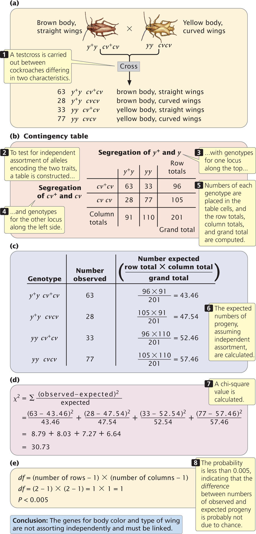
To determine whether the proportions of progeny with genotypes at the two loci are independent, we first construct a table of the observed numbers of progeny, somewhat like a Punnett square, except that we put the genotypes that result from the segregation of alleles at one locus along the top and the genotypes that result from the segregation of alleles at the other locus along the side (Figure 7.10b). Next, we compute the total for each row, the total for each column, and the grand total (the sum of all row totals or the sum of all column totals, which should be the same). These totals will be used to compute the expected values for the chi-square test of independence.
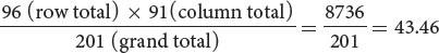
Our next step is to compute the expected values for each combination of genotypes (each cell in the table) with the assumption that the segregation of alleles at the y locus is independent of the segregation of alleles at the cv locus. If the segregation of alleles at each locus is independent, the expected number in each cell can be computed with the following formula:
178
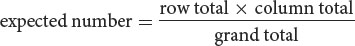
For the cell of the table corresponding to genotype y+y cv+cv (the upper-left-hand cell of the table in Figure 7.10b) the expected number is:
With the use of this method, the expected numbers for each cell are given in Figure 7.10c.
We now calculate a chi-square value by using the same formula that we used for the chi-square goodness-of-fit test in Chapter 3:
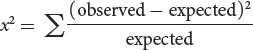
Recall that Σ means “sum” and that we are adding together the (observed −
expected)2/expected value for each type of progeny. With the observed and expected numbers of cockroaches from the testcross, the calculated chi-square value is 30.73 (Figure 7.10d).
To determine the probability associated with this chi-square value, we need the degrees of freedom. Recall from Chapter 3 that the degrees of freedom are the number of ways in which the observed classes are free to vary from the expected values. In general, for the chi-square test of independence, the degrees of freedom equal the number of rows in the table minus 1 multiplied by the number of columns in the table minus 1 (Figure 7.10e), or
df = (number of rows − 1) × (number of columns − 1)
In our example, there are two rows and two columns, and so the degrees of freedom are:
df = (2 − 1) × (2 − 1) = 1 × 1 = 1
Therefore, our calculated chi-square value is 30.73, with 1 degree of freedom. We can use Table 3.7 to find the associated probability. Looking at Table 3.7, we find that our calculated chi-square value is larger than the largest chi-square value given for 1 degree of freedom, which has a probability of 0.005. Thus, our calculated chi-square value has a probability less than 0.005. This very small probability indicates that the genotypes are not in the proportions that we would expect if independent assortment were taking place. Our conclusion, then, is that these genes are not assorting independently and must be linked. As is the case for the goodness-of-fit chi-square test, geneticists generally consider that any chi-square value for the test of independence with a probability less than 0.05 is significantly different from the expected values and is therefore evidence that the genes are not assorting independently. ![]() TRY PROBLEM 16
TRY PROBLEM 16
Gene Mapping with Recombination Frequencies
Thomas Hunt Morgan and his students developed the idea that physical distances between genes on a chromosome are related to the rates of recombination. They hypothesized that crossover events take place more or less at random up and down the chromosome and that two genes that lie far apart are more likely to undergo a crossover than are two genes that lie close together. They proposed that recombination frequencies could provide a convenient way to determine the order of genes along a chromosome and would give estimates of the relative distances between the genes. Chromosome maps calculated by using the genetic phenomenon of recombination are called genetic maps. In contrast, chromosome maps calculated by using physical distances along the chromosome (often expressed as numbers of base pairs) are called physical maps.
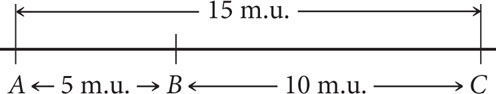
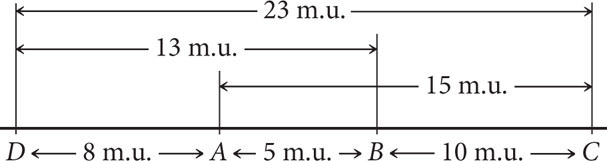
Distances on genetic maps are measured in map units (abbreviated m.u.); one map unit equals 1% recombination. Map units are also called centiMorgans (cM), in honor of Thomas Hunt Morgan. Genetic distances measured with recombination rates are approximately additive: if the distance from gene A to gene B is 5 m.u., the distance from gene B to gene C is 10 m.u., and the distance from gene A to gene C is 15 m.u., then gene B must be located between genes A and C. On the basis of the map distances just given, we can draw a simple genetic map for genes A, B, and C, as shown here:
We could just as plausibly draw this map with C on the left and A on the right:
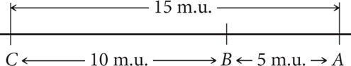
Both maps are correct and equivalent because, with information about the relative positions of only three genes, the most that we can determine is which gene lies in the middle. If we obtained distances to an additional gene, then we could position A and C relative to that gene. An additional gene D, examined through genetic crosses, might yield the following recombination frequencies:
| Gene pair | Recombination frequency (%) |
|---|---|
| A and D | 8 |
| B and D | 13 |
| C and D | 23 |
179
Notice that C and D exhibit the highest percentage of recombination; therefore, C and D must be farthest apart, with genes A and B between them. Using the recombination frequencies and remembering that 1 m.u. = 1% recombination, we can now add D to our map:
By doing a series of crosses between pairs of genes, we can construct genetic maps showing the linkage arrangements of a number of genes.
Two points should be emphasized about constructing chromosome maps from recombination frequencies. First, recall that we cannot distinguish between genes on different chromosomes and genes located far apart on the same chromosome. If genes exhibit 50% recombination, the most that can be said about them is that they belong to different linkage groups, either on different chromosomes or far apart on the same chromosome.
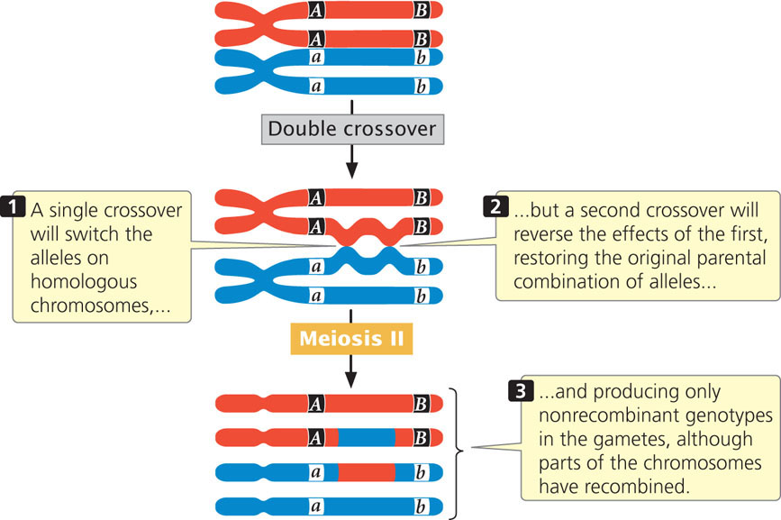
The second point is that a testcross for two genes that are far apart on the same chromosome tends to underestimate the true physical distance because the cross does not reveal double crossovers that might take place between the two genes (Figure 7.11). A double crossover arises when two separate crossover events take place between two loci. (For now, we will consider only double crossovers that take place between two of the four chromatids of a homologous pair—a two-strand double crossover. Double crossovers that take place among three and four chromatids will be considered later, in the section on Effects of Multiple Crossovers.) Whereas a single crossover produces combinations of alleles that were not present on the original parental chromosomes, a second crossover between the same two genes reverses the effects of the first, thus restoring the original parental combination of alleles (see Figure 7.11). We therefore cannot distinguish between the progeny produced by two-strand double crossovers and the progeny produced when there is no crossing over at all. As we shall see in the next section, we can detect double crossovers if we examine a third gene that lies between the two crossovers. Because double crossovers between two genes go undetected, map distances will be underestimated whenever double crossovers take place. Double crossovers are more frequent between genes that are far apart; therefore genetic maps based on short distances are usually more accurate than those based on longer distances.
CONCEPTS
A genetic map provides the order of the genes on a chromosome and the approximate distances from one gene to another based on recombination frequencies. In genetic maps, 1% recombination equals 1 map unit, or 1 centiMorgan. Double crossovers between two genes go undetected, so map distances between distant genes tend to underestimate genetic distances.
CONCEPT CHECK 3
How does a genetic map differ from a physical map?
Constructing a Genetic Map with the Use of Two-Point Testcrosses
Genetic maps can be constructed by conducting a series of testcrosses. In each testcross, one of the parents is heterozygous for a different pair of genes, and recombination frequencies are calculated between pairs of genes. A testcross between two genes is called a two-point testcross, or a two-point cross. Suppose that we carried out a series of two-point crosses for four genes, a, b, c, and d, and obtained the following recombination frequencies:
180
| Gene loci in testcross | Recombination frequency (%) |
|---|---|
| a and b | 50 |
| a and c | 50 |
| a and d | 50 |
| b and c | 20 |
| b and d | 10 |
| c and d | 28 |
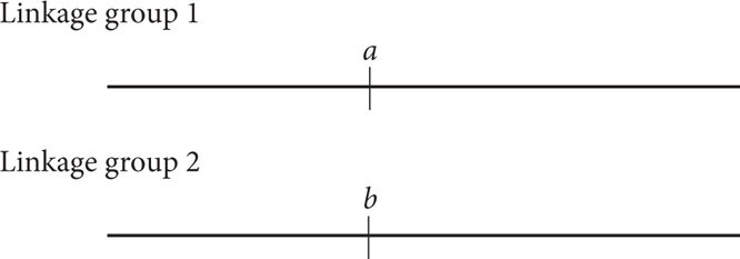
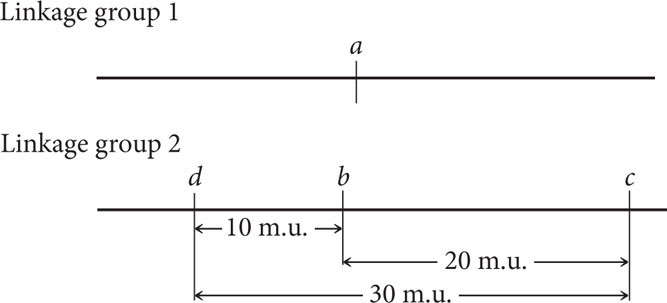
We can begin constructing a genetic map for these genes by considering the recombination frequencies for each pair of genes. The recombination frequency between a and b is 50%, which is the recombination frequency expected with independent assortment. Therefore, genes a and b may either be on different chromosomes or be very far apart on the same chromosome; we will place them in different linkage groups with the understanding that they may or may not be on the same chromosome:
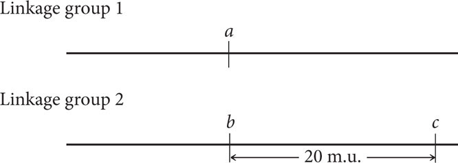
The recombination frequency between a and c is 50%, indicating that they, too, are in different linkage groups. The recombination frequency between b and c is 20%, so these genes are linked and separated by 20 map units:
The recombination frequency between a and d is 50%, indicating that these genes belong to different linkage groups, whereas genes b and d are linked, with a recombination frequency of 10%. To decide whether gene d is 10 m.u. to the left or to the right of gene b, we must consult the c-to-d distance. If gene d is 10 m.u. to the left of gene b, then the distance between d and c should be approximately the sum of the distance between b and c and between c and d: 20 m.u. + 10 m.u. = 30 m.u. If, on the other hand, gene d lies to the right of gene b, then the distance between gene d and gene c will be much shorter, approximately 20 m.u. − 10 m.u. = 10 m.u. The summed distances will be only approximate because any double crossovers between the two genes will be missed and the map distance will be underestimated.
By examining the recombination frequency between c and d, we can distinguish between these two possibilities. The recombination frequency between c and d is 28%, so gene d must lie to the left of gene b. Notice that the sum of the recombination frequency between d and b (10%) and between b and c (20%) is greater than the recombination frequency between d and c (28%). As already discussed, this discrepancy arises because double crossovers between the two outer genes go undetected, causing an underestimation of the true map distance. The genetic map of these genes is now complete:
![]() TRY PROBLEM 27
TRY PROBLEM 27