7.3 A Three-Point Testcross Can Be Used to Map Three Linked Genes
While genetic maps can be constructed from a series of testcrosses for pairs of genes, this approach is not particularly efficient because numerous two-point crosses must be carried out to establish the order of the genes and because double crossovers are missed. A more efficient mapping technique is a testcross for three genes—a three-point testcross, or three-point cross. With a three-point cross, the order of the three genes can be established in a single set of progeny and some double crossovers can usually be detected, providing more-accurate map distances.
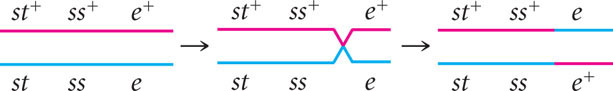
Consider what happens when crossing over takes place among three hypothetical linked genes. Figure 7.12 illustrates a pair of homologous chromosomes of an individual that is heterozygous at three loci (Aa Bb Cc). Notice that the genes are in the coupling configuration; all the dominant alleles are on one chromosome ( A B C ) and all the recessive alleles are on the other chromosome ( a b c ). Three types of crossover events can take place between these three genes: two types of single crossovers (see Figure 7.12a and b) and a double crossover (see Figure 7.12c). In each type of crossover, two of the resulting chromosomes are recombinants and two are nonrecombinants.
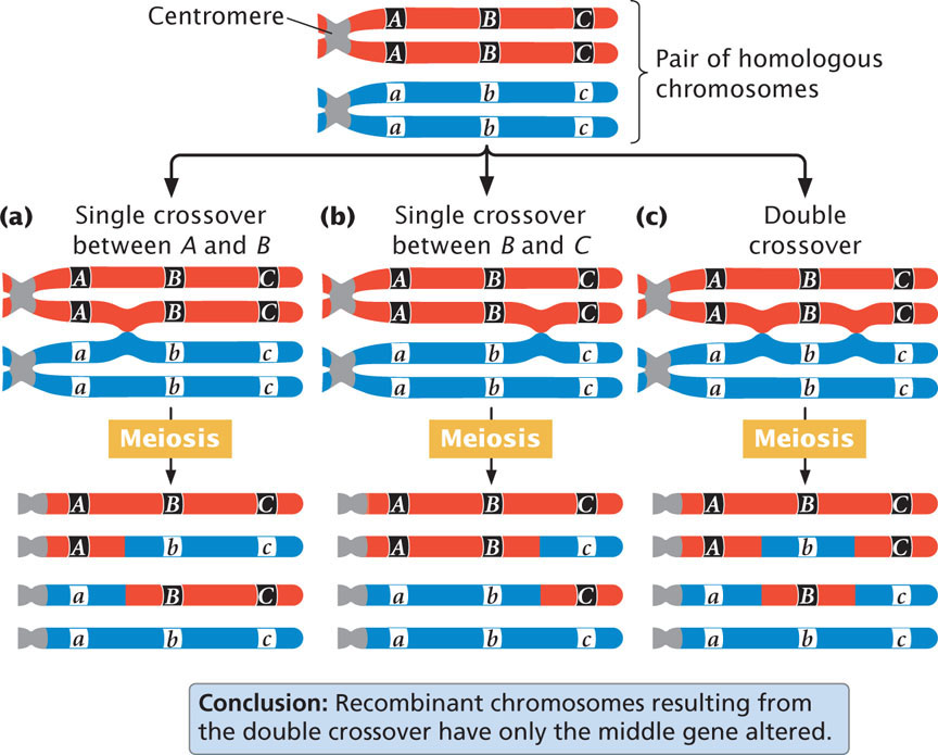
Notice that, in the recombinant chromosomes resulting from the double crossover, the outer two alleles are the same as in the nonrecombinants, but the middle allele is different. This result provides us with an important clue about the order of the genes. In progeny that result from a double crossover, only the middle allele should differ from the alleles present in the nonrecombinant progeny.
181
Constructing a Genetic Map with the Three-Point Testcross
To examine gene mapping with a three-point testcross, we will consider three recessive mutations in the fruit fly Drosophila melanogaster. In this species, scarlet eyes (st) are recessive to wild-type red eyes (st+), ebony body color (e) is recessive to wild-type gray body color (e+), and spineless (ss)—that is, the presence of small bristles—is recessive to wild-type normal bristles (ss+). The loci encoding these three characteristics are linked and located on chromosome 3.
We will refer to these three loci as st, e, and ss, but keep in mind that either the recessive alleles (st, e, and ss) or the dominant alleles (st+, e+, and ss+) may be present at each locus. So, when we say that there are 10 m.u. between st and ss, we mean that there are 10 m.u. between the loci at which mutations st and ss occur; we could just as easily say that there are 10 m.u. between st+ and ss+.
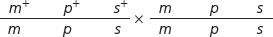
To map these genes, we need to determine their order on the chromosome and the genetic distances between them. First, we must set up a three-point testcross: a cross between a fly heterozygous at all three loci and a fly homozygous for recessive alleles at all three loci. To produce flies heterozygous for all three loci, we might cross a stock of flies that are homozygous for wild-type alleles at all three loci with flies that are homozygous for recessive alleles at all three loci:
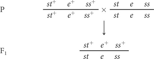
The order of the genes has been arbitrarily assigned because, at this point, we do not know which one is the middle gene. Additionally, the alleles in these heterozygotes are in coupling configuration (because all the wild-type dominant alleles were inherited from one parent and all the recessive mutations from the other parent), although the testcross can also be done with alleles in repulsion.
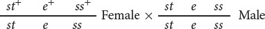
In the three-point testcross, we cross the F1 heterozygotes with flies that are homozygous for all three recessive mutations. In many organisms, it makes no difference whether the heterozygous parent in the testcross is male or female (provided that the genes are autosomal) but, in Drosophila, no crossing over takes place in males. Because crossing over in the heterozygous parent is essential for determining recombination frequencies, the heterozygous flies in our testcross must be female. So we mate female F1 flies that are heterozygous for all three traits with male flies that are homozygous for all the recessive traits:
182
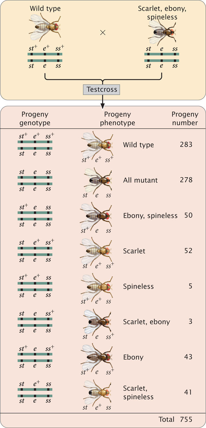
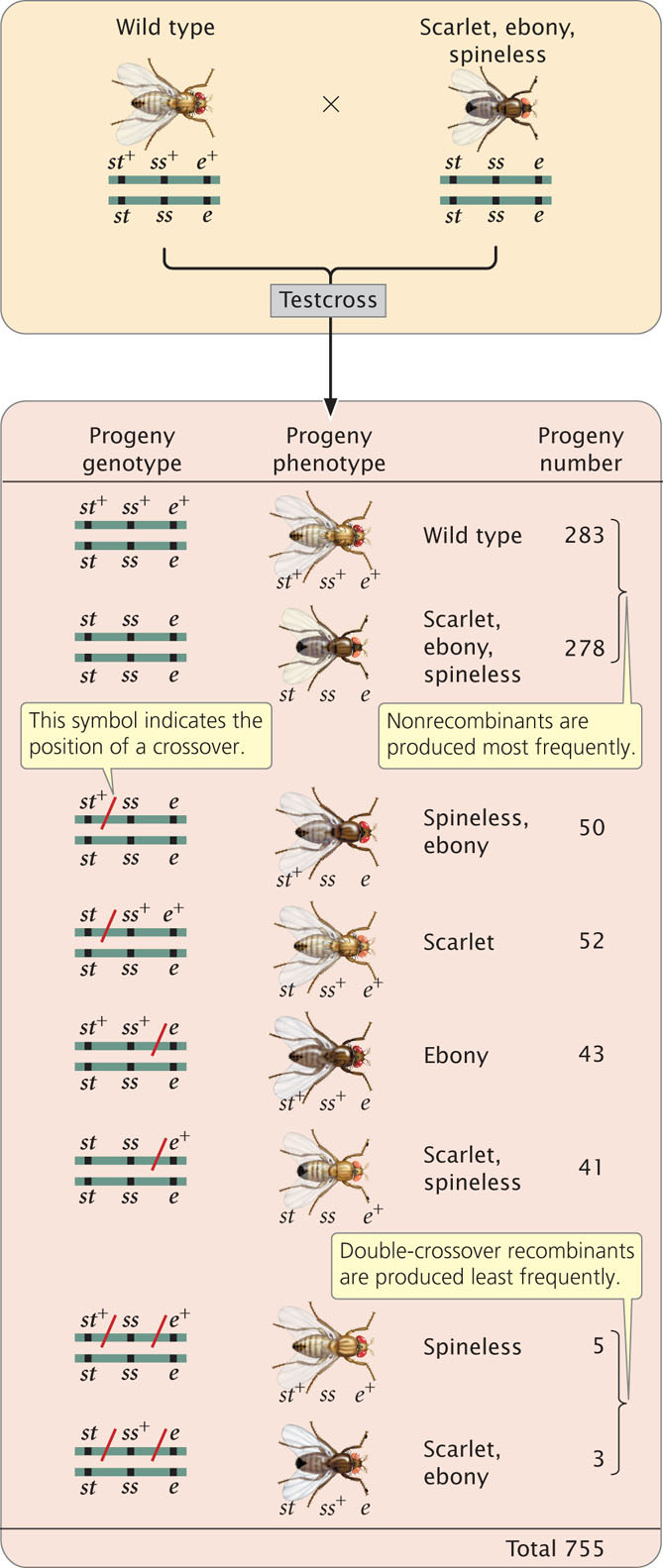
The progeny produced from this cross are listed in Figure 7.13. For each locus, two classes of progeny are produced: progeny that are heterozygous, displaying the dominant trait, and progeny that are homozygous, displaying the recessive trait. With two classes of progeny possible for each of the three loci, there will be 23 = 8 classes of phenotypes possible in the progeny. In this example, all eight phenotypic classes are present but, in some three-point crosses, one or more of the phenotypes may be missing if the number of progeny is limited. Nevertheless, the absence of a particular class can provide important information about which combination of traits is least frequent and, ultimately, about the order of the genes, as we will see.
To map the genes, we need information about where and how often crossing over has taken place. In the homozygous recessive parent, the two alleles at each locus are the same, and so crossing over will have no effect on the types of gametes produced; with or without crossing over, all gametes from this parent have a chromosome with three recessive alleles ( st e ss ). In contrast, the heterozygous parent has different alleles on its two chromosomes, and so crossing over can be detected. The information that we need for mapping, therefore, comes entirely from the gametes produced by the heterozygous parent. Because chromosomes contributed by the homozygous parent carry only recessive alleles, whatever alleles are present on the chromosome contributed by the heterozygous parent will be expressed in the progeny.
As a shortcut, we often do not write out the complete genotypes of the testcross progeny, listing instead only the alleles expressed in the phenotype, which are the alleles inherited from the heterozygous parent. This convention is used in the discussion that follows.
CONCEPTS
To map genes, information about the location and number of crossovers in the gametes that produced the progeny of a cross is needed. An efficient way to obtain this information is to use a three-point testcross, in which an individual heterozygous at three linked loci is crossed with an individual that is homozygous recessive at the three loci.
 CONCEPT CHECK 4
Write the genotypes of all recombinant and nonrecombinant progeny expected from the following three-point cross:
Determining the Gene Order
The first task in mapping the genes is to determine their order on the chromosome. In Figure 7.13, we arbitrarily listed the loci in the order st, e, ss, but we had no way of knowing which of the three loci was between the other two. We can now identify the middle locus by examining the double-crossover progeny.
First, determine which progeny are the nonrecombinants; they will be the two most-numerous classes of progeny (even if crossing over takes place in every meiosis, the nonrecombinants will constitute at least 50% of the progeny). Among the progeny of the testcross in Figure 7.13, the most numerous are those with all three dominant traits ( st+ e+ ss+ ) and those with all three recessive traits ( st e ss ).
183
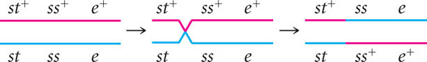
Next, identify the double-crossover progeny. These progeny should always have the two least-numerous phenotypes, because the probability of a double crossover is always less than the probability of a single crossover. The least-common progeny among those listed in Figure 7.13 are progeny with spineless bristles, ( st+ e+ ss ) and progeny with scarlet eyes and ebony body ( st e ss+ ), so they are the double-crossover progeny.
Three orders of genes on the chromosome are possible: the eye-color locus could be in the middle ( e st ss ), the body-color locus could be in the middle ( st e ss ), or the bristle locus could be in the middle ( st ss e ). To determine which gene is in the middle, we can draw the chromosomes of the heterozygous parent with all three possible gene orders and then see if a double crossover produces the combination of genes observed in the double-crossover progeny. The three possible gene orders and the types of progeny produced by their double crossovers are:
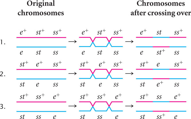
The only gene order that produces chromosomes with the set of alleles observed in the least-numerous progeny or double crossovers ( st+ e+ ss and st e ss+ in Figure 7.13) is the one in which the ss locus for bristles lies in the middle (gene-order 3). Therefore, this order ( st ss e ) must be the correct sequence of genes on the chromosome.
With a little practice, we can quickly determine which locus is in the middle without writing out all the gene orders. The phenotypes of the progeny are expressions of the alleles inherited from the heterozygous parent. Recall that when we looked at the results of double crossovers (see Figure 7.12) only the alleles at the middle locus differed from the nonrecombinants. If we compare the nonrecombinant progeny with double-crossover progeny, they should differ only in alleles of the middle locus (Table 7.2).
| 1. | Identify the nonrecombinant progeny (two most-numerous phenotypes). |
| 2. | Identify the double-crossover progeny (two least-numerous phenotypes). |
| 3. | Compare the phenotype of double-crossover progeny with the phenotype of nonrecombinant progeny. They should be alike in two characteristics and differ in one. |
| 4. | The characteristic that differs between the double crossover and the nonrecombinant progeny is encoded by the middle gene. |
Let’s compare the alleles in the double-crossover progeny st+ e+ ss with those in the nonrecombinant progeny st+ e+ ss+. We see that both have an allele for red eyes (st+) and both have an allele for gray body (e+), but the nonrecombinants have an allele for normal bristles (ss+), whereas the double crossovers have an allele for spineless bristles (ss). Because the bristle locus is the only one that differs, it must lie in the middle. We would obtain the same results if we compared the other class of double-crossover progeny ( st e ss+ ) with other nonrecombinant progeny ( st e ss ). Again, the only locus that differs is the one for bristles. Don’t forget that the nonrecombinants and the double crossovers should differ at only one locus; if they differ at two loci, the wrong classes of progeny are being compared.  Animation 7.1 illustrates how to determine the order of the three linked genes.
CONCEPTS
To determine the middle locus in a three-point cross, compare the double-crossover progeny with the nonrecombinant progeny. The double crossovers will be the two least-common classes of phenotypes; the nonrecombinants will be the two most-common classes of phenotypes. The double-crossover progeny should have the same alleles as the nonrecombinant types at two loci and different alleles at the locus in the middle.
CONCEPT CHECK 5
A three-point test cross is carried out between three linked genes. The resulting nonrecombinant progeny are s+ r+ c+ and s r c and the double-crossover progeny are s r c+ and s+ r+ c. Which is the middle locus?
Determining the Locations of Crossovers
When we know the correct order of the loci on the chromosome, we should rewrite the phenotypes of the testcross progeny in Figure 7.13 with the alleles in the correct order so that we can determine where crossovers have taken place (Figure 7.14).
Among the eight classes of progeny, we have already identified two classes as nonrecombinants ( st+ ss+ e+ and st ss e ) and two classes as double crossovers ( st+ ss e+ and st ss+ e ). The other four classes include progeny that resulted from a chromosome that underwent a single crossover: two underwent single crossovers between st and ss, and two underwent single crossovers between ss and e.
184
To determine where the crossovers took place in these progeny, compare the alleles found in the single-crossover progeny with those found in the nonrecombinants, just as we did for the double crossovers. For example, consider progeny with chromosome st+ ss e . The first allele (st+) came from the nonrecombinant chromosome st+ ss+ e+ and the other two alleles (ss and e) must have come from the other nonrecombinant chromosome st ss e through crossing over:
This same crossover also produces the st ss+ e+ progeny.
This method can also be used to determine the location of crossing over in the other two types of single-crossover progeny. Crossing over between ss and e produces st+ ss+ e and st ss e+ chromosomes:
We now know the locations of all the crossovers; their locations are marked with a slash in Figure 7.14.
Calculating the Recombination Frequencies
Next we can determine the map distances, which are based on the frequencies of recombination. We calculate recombination frequency by adding up all of the recombinant progeny, dividing this number by the total number of progeny from the cross, and multiplying the number obtained by 100%. To determine the map distances accurately, we must include all crossovers (both single and double) that take place between two genes.
Recombinant progeny that possess a chromosome that underwent crossing over between the eye-color locus (st) and the bristle locus (ss) include the single crossovers ( st+ / ss e and st / ss+ e+ ) and the two double crossovers ( st+ / ss / e and); see Figure 7.14. There are a total of 755 progeny; so the recombination frequency between ss and st is:
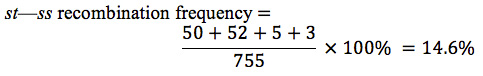
The distance between the st and ss loci can be expressed as 14.6 m.u.
185
The map distance between the bristle locus (ss) and the body locus (e) is determined in the same manner. The recombinant progeny that possess a crossover between ss and e are the single crossovers st+ ss+ / e and st ss / e+ and the double crossovers st+ / ss / e+ and st / ss+ / e . The recombination frequency is:
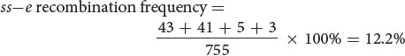
Thus, the map distance between ss and e is 12.2 m.u.
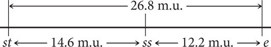
Finally, calculate the map distance between the outer two loci, st and e. This map distance can be obtained by summing the map distances between st and ss and between ss and e (14.6 m.u. + 12.2 m.u. = 26.8 m.u.). We can now use the map distances to draw a map of the three genes on the chromosome:
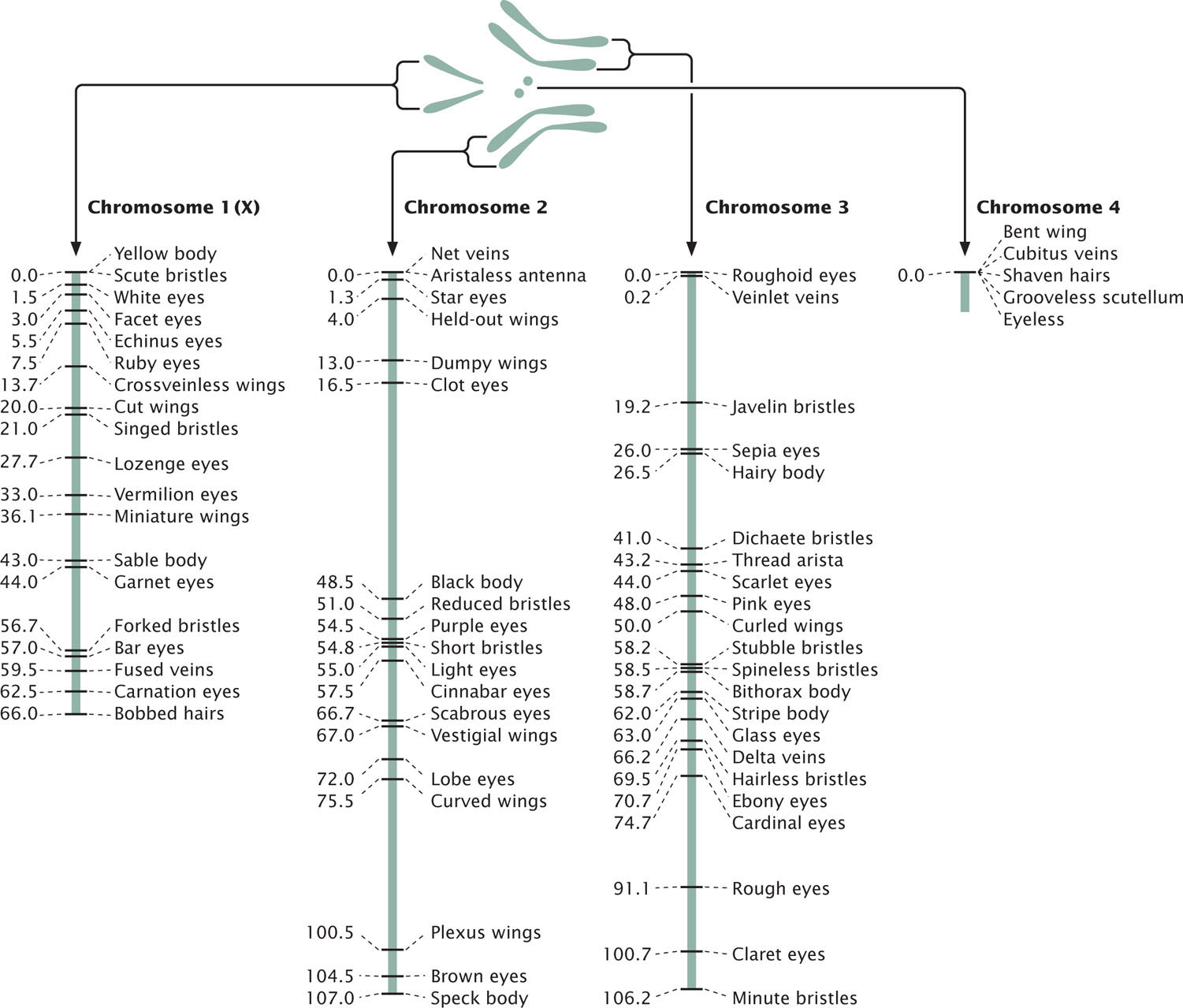
A genetic map of D. melanogaster is illustrated in Figure 7.15.
Interference and the Coefficient of Coincidence
Map distances give us information not only about the distances that separate genes, but also about the proportions of recombinant and nonrecombinant gametes that will be produced in a cross. For example, knowing that genes st and ss on the third chromosome of D. melanogaster are separated by a distance of 14.6 m.u. tells us that 14.6% of the gametes produced by a fly heterozygous at these two loci will be recombinants. Similarly, 12.2% of the gametes from a fly heterozygous for ss and e will be recombinants.
186
Theoretically, we should be able to calculate the proportion of double-recombinant gametes by using the multiplication rule of probability (see Chapter 3). Applying this rule, we should find that the proportion (probability) of gametes with double crossovers between st and e is equal to the probability of recombination between st and ss multiplied by the probability of recombination between ss and e, or 0.146 × 0.122 = 0.0178. Multiplying this probability by the total number of progeny gives us the expected number of double-crossover progeny from the cross: 0.0178 × 755 = 13.4. Only 8 double crossovers—considerably fewer than the 13 expected—were observed in the progeny of the cross (see Figure 7.14).
This phenomenon is common in eukaryotic organisms. The calculation assumes that each crossover event is independent and that the occurrence of one crossover does not influence the occurrence of another. But crossovers are frequently not independent events: the occurrence of one crossover tends to inhibit additional crossovers in the same region of the chromosome, and so double crossovers are less frequent than expected.
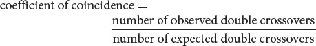
The degree to which one crossover interferes with additional crossovers in the same region is termed the interference. To calculate the interference, we first determine the coefficient of coincidence, which is the ratio of observed double crossovers to expected double crossovers:
For the loci that we mapped on the third chromosome of D. melanogaster (see Figure 7.14), we find that the
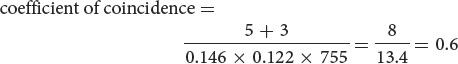
which indicates that we are actually observing only 60% of the double crossovers that we expected on the basis of the single-crossover frequencies. The interference is calculated as
interference = 1 − coefficient of coincidence
So the interference for our three-point cross is:
interference = 1 − 0.6 = 0.4
This value of interference tells us that 40% of the double-crossover progeny expected will not be observed, because of interference. When interference is complete and no double-crossover progeny are observed, the coefficient of coincidence is 0 and the interference is 1.
Sometimes a crossover increases the probability of another crossover taking place nearby and we see more double-crossover progeny than expected. In this case, the coefficient of coincidence is greater than 1 and the interference is negative.
Most eukaryotic organisms exhibit interference, which causes crossovers to be more widely spaced than would be expected on a random basis. Interference was first observed in crosses of Drosophila in the early 1900s and yet, despite years of study, the mechanism by which interference occurs is still not well understood. One proposed model of interference suggests that crossovers occur when stress builds up along the chromosome. Under this model, a crossover releases stress for some distance along the chromosome. Because a crossover relieves the stress that causes crossovers, additional crossovers are less likely to occur in the same area. ![]() TRY PROBLEM 29
TRY PROBLEM 29
CONCEPTS
The coefficient of coincidence equals the number of double crossovers observed divided by the number of double crossovers expected on the basis of the single-crossover frequencies. The interference equals 1 − the coefficient of coincidence; it indicates the degree to which one crossover interferes with additional crossovers.
CONCEPT CHECK 6
In analyzing the results of a three-point testcross, a student determines that the interference is −0.23. What does this negative interference value indicate?
- Fewer double crossovers took place than expected on the basis of single-crossover frequencies.
- More double crossovers took place than expected on the basis of single-crossover frequencies.
- Fewer single crossovers took place than expected.
- A crossover in one region interferes with additional crossovers in the same region.
CONNECTING CONCEPTS: Stepping Through the Three-Point Cross
We have now examined the three-point cross in considerable detail and have seen how the information derived from the cross can be used to map a series of three linked genes. Let’s briefly review the steps required to map genes from a three-point cross.
- 1. Write out the phenotypes and numbers of progeny produced in the three-point cross. The progeny phenotypes will be easier to interpret if you use allelic symbols for the traits (such as st+ e+ ss).
- 2. Write out the genotypes of the original parents used to produce the triply heterozygous individual in the testcross and, if known, the arrangement (coupling or repulsion) of the alleles on their chromosomes.
- 3. Determine which phenotypic classes among the progeny are the nonrecombinants and which are the double crossovers. The nonrecombinants will be the two most-common phenotypes; double crossovers will be the two least-common phenotypes.
- 4. Determine which locus lies in the middle. Compare the alleles present in the double crossovers with those present in the nonrecombinants; each class of double crossovers should be like one of the nonrecombinants for two loci and should differ for one locus. The locus that differs is the middle one.
- 5. Rewrite the phenotypes with the genes in correct order.
- 6. Determine where crossovers must have taken place to give rise to the progeny phenotypes. To do so, compare each phenotype with the phenotype of the nonrecombinant progeny.
- 7. Determine the recombination frequencies. Add the numbers of the progeny that possess a chromosome with a crossover between a pair of loci. Add the double crossovers to this number. Divide this sum by the total number of progeny from the cross, and multiply by 100%; the result is the recombination frequency between the loci, which is the same as the map distance.
- 8. Draw a map of the three loci. Indicate which locus lies in the middle, and indicate the distances between them.
- 9. Determine the coefficient of coincidence and the interference. The coefficient of coincidence is the number of observed double-crossover progeny divided by the number of expected double-crossover progeny. The expected number can be obtained by multiplying the product of the two single-recombination probabilities by the total number of progeny in the cross.
WORKED PROBLEM
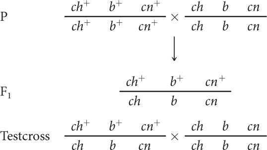
In D. melanogaster, cherub wings (ch), black body (b), and cinnabar eyes (cn) result from recessive alleles that are all located on chromosome 2. A homozygous wild-type fly was mated with a cherub, black, and cinnabar fly, and the resulting F1 females were test-crossed with cherub, black, and cinnabar males. The following progeny were produced from the testcross:
| ch | b+ | cn | 105 |
| ch+ | b+ | cn+ | 750 |
| ch+ | b | cn | 40 |
| ch+ | b+ | cn | 4 |
| ch | b | cn | 753 |
| ch | b+ | cn+ | 41 |
| ch+ | b | cn+ | 102 |
| ch | b | cn+ | 5 |
| Total | 1800 |
- a. Determine the linear order of the genes on the chromosome (which gene is in the middle?).
- b. Calculate the recombinant distances between the three loci.
- c. Determine the coefficient of coincidence and the interference for these three loci.
Solution Strategy
What information is required in your answer to the problem?
The order of the genes on the chromosome, the recombinant distances among the genes, the coefficient of coincidence, and the interference.
What information is provided to solve the problem?
 A homozygous wild-type fly was mated with a cherub, black, and cinnabar fly, and the resulting F1 females were test-crossed with cherub, black, and cinnabar males.
-
The numbers of the different types of flies appearing among the progeny of the test cross.
Solution Steps
- a. We can represent the crosses in this problem as follows:Note that at this point we do not know the order of the genes; we have arbitrarily put b in the middle.
The next step is to determine which of the testcross progeny are nonrecombinants and which are double crossovers. The nonrecombinants should be the most-frequent phenotype, so they must be the progeny with phenotypes encoded by ch+ b+ cn+ and ch b cn. These genotypes are consistent with the genotypes of the parents, given earlier. The double crossovers are the least-frequent phenotypes and are encoded by ch+ b+ cn and ch b cn+.
We can determine the gene order by comparing the alleles present in the double crossovers with those present in the nonrecombinants. The double-crossover progeny should be like one of the nonrecombinants at two loci and unlike it at one locus; the allele that differs should be in the middle. Compare the double-crossover progeny ch b cn+ with the nonrecombinant ch b cn. Both have cherub wings (ch) and black body (b), but the double-crossover progeny have wild-type eyes (cn+), whereas the nonrecombinants have cinnabar eyes (cn). The locus that determines cinnabar eyes must be in the middle.
- b. To calculate the recombination frequencies among the genes, we first write the phenotypes of the progeny with the genes encoding them in the correct order. We have already identified the nonrecombinant and double-crossover progeny, so the other four progeny types must have resulted from single crossovers. To determine where single crossovers took place, we compare the alleles found in the single-crossover progeny with those in the nonrecombinants. Crossing over must have taken place where the alleles switch from those found in one nonrecombinant to those found in the other nonrecombinant. The locations of the crossovers are indicated with a slash:
188
ch cn / b+ 105 single crossover ch+ cn+ b+ 750 nonrecombinant ch+ / cn b 40 single crossover ch+ / cn / b+ 4 double crossover ch cn b 753 nonrecombinant ch / cn+ b+ 41 single crossover ch+ cn+ / b 102 single crossover ch / cn+ / b 5 double crossover Total 1800
Next, we determine the recombination frequencies and draw a genetic map:
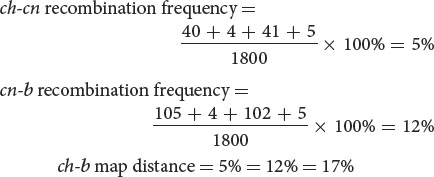
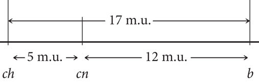
- c. The coefficient of coincidence is the number of observed double crossovers divided by the number of expected double crossovers. The number of expected double crossovers is obtained by multiplying the probability of a crossover between ch and cn (0.05) × the probability of a crossover between cn and b (0.12) × the total number of progeny in the cross (1800):

Finally, the interference is equal to 1 − the coefficient of coincidence:
interference = 1 − 0.83 = 0.17
To increase your skill with three-point crosses, try working Problem 30 at the end of this chapter.
Effect of Multiple Crossovers
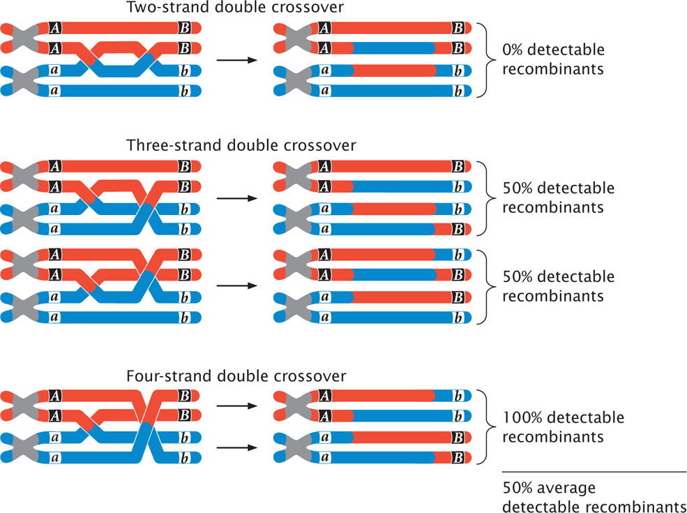
So far, we have examined the effects of double crossovers taking place between only two of the four chromatids (strands) of a homologous pair. These crossovers are called two-strand crossovers. Double crossovers including three and even four of the chromatids of a homologous pair also may take place (Figure 7.16). If we examine only the alleles at loci on either side of both crossover events, two-strand double crossovers result in no new combinations of alleles, and no recombinant gametes are produced (see Figure 7.16). Three-strand double crossovers result in two of the four gametes being recombinant, and four-strand double crossovers result in all four gametes being recombinant. Thus, two-strand double crossovers produce 0% recombination, three-strand double crossovers produce 50% recombination, and four-strand double crossovers produce 100% recombination. The overall result is that all types of double crossovers, taken together, produce an average of 50% recombinant progeny.
189
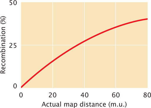
As we have seen, two-strand double crossovers cause alleles on either side of the crossovers to remain the same and produce no recombinant progeny. Three-strand and four-strand crossovers produce recombinant progeny, but these progeny are the same types as those produced by single crossovers. Consequently, some multiple crossovers go undetected when the progeny of a genetic cross are observed. Therefore, map distances based on recombination rates will underestimate the true physical distances between genes because some multiple crossovers are not detected among the progeny of a cross. When genes are very close together, multiple crossovers are unlikely and the distances based on recombination rates accurately correspond to the physical distances on the chromosome. But, as the distance between genes increases, more multiple crossovers are likely and the discrepancy between genetic distances (based on recombination rates) and physical distances increases. To correct for this discrepancy, geneticists have developed mathematical mapping functions, which relate recombination frequencies to actual physical distances between genes (Figure 7.17). Most of these functions are based on the Poisson distribution, which predicts the probability of multiple rare events. With the use of such mapping functions, map distances based on recombination rates can be more accurately estimated.
Mapping Human Genes
Efforts in mapping human genes are hampered by the inability to perform desired crosses and the small number of progeny in most human families. Geneticists are often restricted to analyses of pedigrees, which are often incomplete and provide limited information. Nevertheless, a large number of human traits have been successfully mapped with the use of pedigree data to analyze linkage. Because the number of progeny from any one mating is usually small, data from several families and pedigrees are usually combined to test for independent assortment. The methods used in these types of analysis are complex, but an example will illustrate how linkage can be detected from pedigree data.
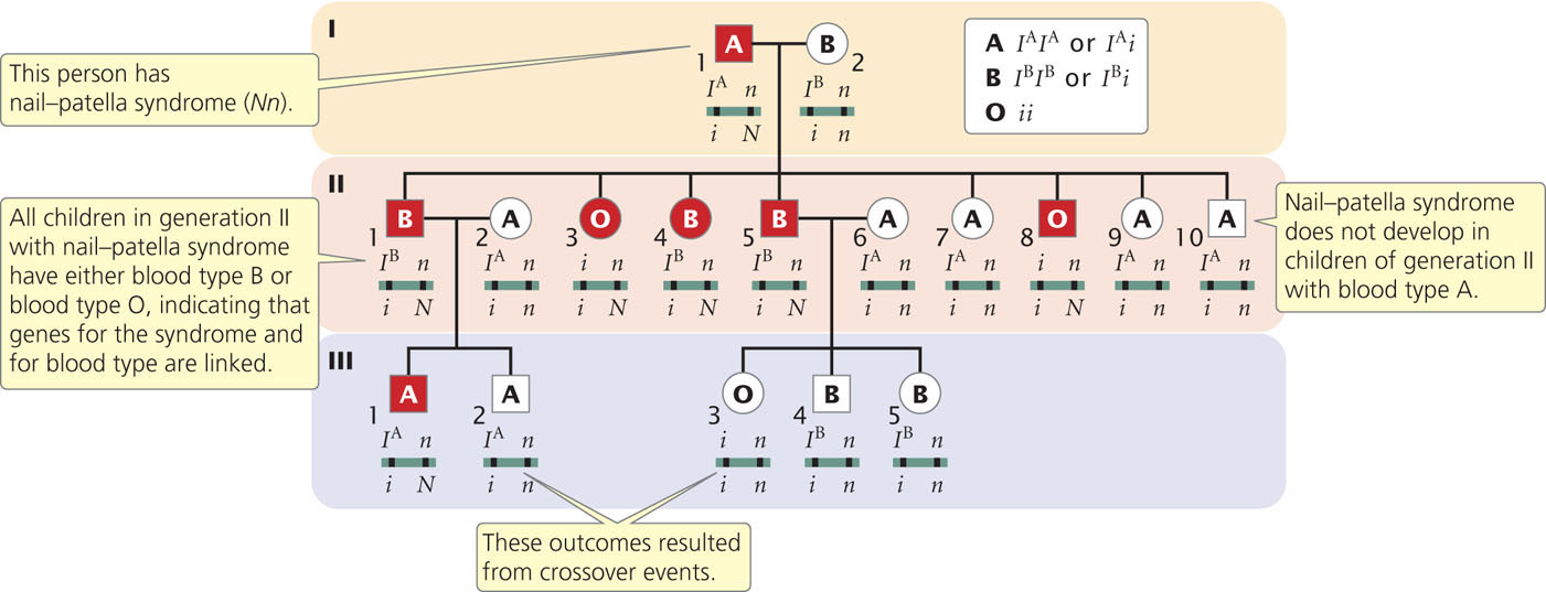
One of the first documented demonstrations of linkage in humans was between the locus for nail–patella syndrome and the locus that determines the ABO blood types. Nail–patella syndrome is an autosomal dominant disorder characterized by abnormal fingernails and absent or rudimentary kneecaps. The ABO blood types are determined by an autosomal locus with multiple alleles (see Chapter 5). Linkage between the genes encoding these traits was established in families in which both traits segregate. Part of one such family is illustrated in Figure 7.18.
190
Nail-patella syndrome is rare, and so we can assume that people who have this trait are heterozygous (Nn); unaffected people are homozygous (nn). The ABO genotypes can be inferred from the phenotypes and the types of offspring produced. Person I-2 in Figure 7.18, for example, has blood-type B, which has two possible genotypes: IBIB or IBi (see Figure 5.6). Because some of her offspring are blood-type O (genotype ii) and must have therefore inherited an i allele from each parent, female I-2 must have genotype IBi. Similarly, the presence of blood-type O offspring in generation II indicates that male I-1, with blood-type A, also must carry an i allele and therefore has genotype IAi. The parents of this family are:
IAi Nn × IBi nn
From generation II, we can see that the genes for nail–patella syndrome and the blood types do not appear to assort independently. All children in generation II with nail-patella syndrome have either blood-type B or blood-type O; all those with blood-type A have normal nails and kneecaps. If the genes encoding nail-patella syndrome and the ABO blood types assorted independently, we would expect that some children in generation II would have blood-type A and nail–patella syndrome, inheriting both the IA and N alleles from their father. This outcome indicates that the arrangements of the alleles on the chromosomes of the crossed parents are:
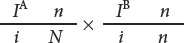
The pedigree indicates that there is no recombination among the offspring (generation II) of these parents, but there are two instances of recombination among the persons in generation III. Persons II-1 and II-2 have the following genotypes:
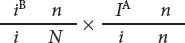
Their child III-2 has blood-type A and does not have nail-patella syndrome; so he must have genotype

and must have inherited both the i and the n alleles from his father. These alleles are on different chromosomes in the father; so crossing over must have taken place. Crossing over also must have taken place to produce child III-3.
In the pedigree of Figure 7.18, 13 children are from matings in which the genes encoding nail–patella syndrome and ABO blood types segregate; two of them are recombinants. On this basis, we might assume that the loci for nail-patella syndrome and ABO blood types are linked, with a recombination frequency of  = 0.154. However, it is possible that the genes are assorting independently and that the small number of children just makes it seem as though the genes are linked. To determine the probability that genes are actually linked, geneticists often calculate lod (logarithm of odds) scores.
To obtain a lod score, we calculate both the probability of obtaining the observed results with the assumption that the genes are linked with a specified degree of recombination and the probability of obtaining the observed results with the assumption of independent assortment. We then determine the ratio of these two probabilities, and the logarithm of this ratio is the lod score. Suppose that the probability of obtaining a particular set of observations with the assumption of linkage and a certain recombination frequency is 0.1 and that the probability of obtaining the same observations with the assumption of independent assortment is 0.0001. The ratio of these two probabilities is  = 1000, the logarithm of which (the lod score) is 3. Thus, linkage with the specified recombination is 1000 times as likely as independent assortment to produce what was observed. A lod score of 3 or higher is usually considered convincing evidence for linkage.
 ![]() TRY PROBLEM 36
TRY PROBLEM 36
Mapping with Molecular Markers
For many years, gene mapping was limited in most organisms by the availability of genetic markers—variable genes with easily observable phenotypes for which inheritance could be studied. Traditional genetic markers include genes that encode easily observable characteristics such as flower color, seed shape, blood types, or biochemical differences. The paucity of these types of characteristics in many organisms limited mapping efforts.
In the 1980s, new molecular techniques made it possible to examine variations in DNA itself, providing an almost unlimited number of genetic markers that can be used for creating genetic maps and studying linkage relations. The earliest of these markers consisted of restriction fragment length polymorphisms (RFLPs), which are variations in DNA sequence detected by cutting the DNA with restriction enzymes (see Chapter 19). Later, methods were developed for detecting variable numbers of short DNA sequences repeated in tandem, called microsatellites. Now DNA sequencing allows the direct detection of individual variations in the DNA nucleotides. All of these methods have expanded the availability of genetic markers and greatly facilitated the creation of genetic maps.
Gene mapping with molecular markers is done essentially in the same manner as mapping performed with traditional phenotypic markers: the cosegregation of two or more markers is studied, and map distances are based on the rates of recombination between markers. These methods and their use in mapping are presented in more detail in Chapters 19 and 20.
191
Genes Can Be Located with Genomewide Association Studies
The traditional approach to mapping genes, which we have learned in this chapter, is to examine progeny phenotypes in genetic crosses or among individuals in a pedigree, looking for associations between the inheritance of a particular phenotype and the inheritance of alleles at other loci. This type of gene mapping is called linkage analysis, because it is based on the detection of physical linkage between genes, as measured by the rate of recombination, in progeny from a cross. Linkage analysis has been a powerful tool in the genetic analysis of many different types of organisms, including fruit flies, corn, mice, and humans.
Another alternative approach to mapping genes is to conduct genomewide association studies, looking for nonrandom associations between the presence of a trait and alleles at many different loci scattered across the genome. Unlike linkage analysis, this approach does not trace the inheritance of genetic markers and a trait in a genetic cross or family. Rather, it looks for associations between traits and particular suites of alleles in a population.
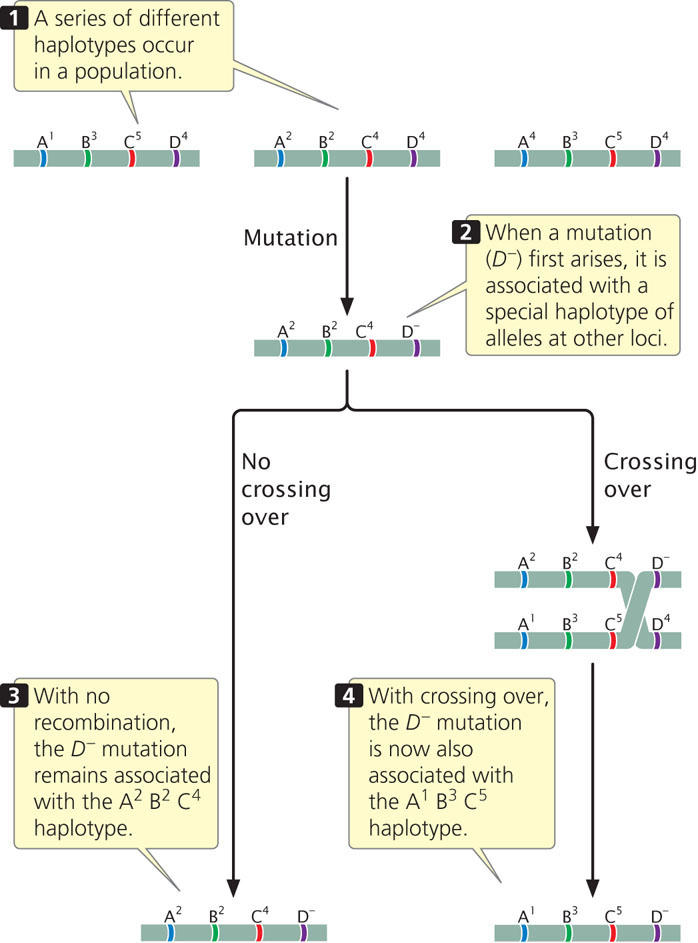
Imagine that we are interested in finding genes that contribute to bipolar disease, a psychiatric illness characterized by severe depression and mania. When a mutation that predisposes a person to bipolar disease first arises in a population, it will occur on a particular chromosome and will be associated with a specific set of alleles on that chromosome. In the example illustrated in Figure 7.19, the D− mutation first arises on a chromosome that has alleles A2, B2, and C4, and therefore the D− mutation is initially linked to A2, B2, and C4 alleles. A specific set of linked alleles such as this is called a haplotype, and the nonrandom association between alleles in a haplotype is called linkage disequilibrium. Because of the physical linkage between the bipolar mutation and the other alleles of the haplotype, bipolar illness and the haplotype will tend to be inherited together. Crossing over, however, breaks up the association between the alleles of the haplotype (see Figure 7.19), reducing the linkage disequilibrium between them. How long the linkage disequilibrium persists over evolutionary time depends on the amount of recombination between alleles at different loci. When the loci are far apart, linkage disequilibrium breaks down quickly; when the loci are close together, crossing over is less common and linkage disequilibrium will persist longer. The important point is that linkage disequilibrium—the nonrandom association between alleles—provides information about the distance between genes. A strong association between a trait such as bipolar illness and a set of linked genetic markers indicates that one or more genes contributing to bipolar illness are likely to be near the genetic markers.
In recent years, geneticists have mapped millions of genetic variants called single-nucleotide polymorphisms (SNPs), which are positions in the genome where people vary in a single nucleotide base (see Chapter 20). Recall that SNPs were used in a linkage analysis that located the gene responsible for pattern baldness, discussed in the introduction to this chapter. It is now possible to quickly and inexpensively genotype people for hundreds of thousands or millions of SNPs. This genotyping has provided genetic markers needed for conducting genomewide association studies, in which SNP haplotypes of people who have a particular disease, such as bipolar illness, are compared with the haplotypes of healthy people. Nonrandom associations between SNPs and the disease suggest that one or more genes that contribute to the disease are closely linked to the SNPs. Genomewide association studies do not usually locate specific genes: rather, they associate the inheritance of a trait or disease with a specific chromosomal region. After such an association has been established, geneticists can examine the chromosomal region for genes that might be responsible for the trait. Genomewide association studies have been instrumental in the discovery of genes or chromosomal regions that affect a number of genetic diseases and important human traits, including bipolar disease, height, skin pigmentation, eye color, body weight, coronary artery disease, blood-lipid concentrations, diabetes, heart attacks, bone density, and glaucoma, among others.
192
CONCEPTS
The development of molecular techniques for examining variation in DNA sequences has provided a large number of genetic markers that can be used to create genetic maps and study linkage relations. Genomewide association studies examine the nonrandom association of genetic markers and phenotypes to locate genes that contribute to the expression of traits.