To determine how much of the phenotypic variation in a population is due to genetic factors and how much is due to environmental factors, we must first have some quantitative measure of the phenotype under consideration. Consider a population of wild plants that differ in size. We could collect a representative sample of plants from the population, weigh each plant in the sample, and calculate the mean and variance of plant weight. This phenotypic variance is represented by V_P.

COMPONENTS OF PHENOTYPIC VARIANCE First, some of the phenotypic variance may be due to differences in genotypes among individual members of the population. These differences are termed the genetic variance and are represented by V_G.

Second, some of the differences in phenotype may be due to environmental differences among the plants; these differences are termed the environmental variance, V_E. Environmental variance includes differences in environmental factors such as the amount of light or water that the plant receives; it also includes random differences in development that cannot be attributed to any specific factor. Any variation in phenotype that is not inherited is, by definition, a part of the environmental variance.

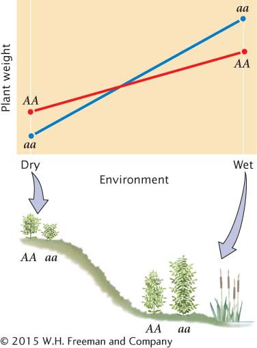
Third, genetic–environmental interaction variance (V_GE) arises when the effect of a gene depends on the specific environment in which it is found. An example is shown in Figure 17.11. In a dry environment, genotype AA produces a plant that averages 12 g in weight, and genotype aa produces a smaller plant that averages 10 g. In a wet environment, genotype aa produces the larger plant, averaging 24 g in weight, whereas genotype AA produces a plant that averages 20 g. In this example, there are clearly differences in the two environments: both genotypes produce heavier plants in the wet environment. There are also differences in the weights of the two genotypes, but the relative performances of the two genotypes depend on whether the plants are grown in a wet or a dry environment. In this case, the influences on phenotype cannot be neatly allocated into genetic and environmental components because the expression of the genotype depends on the environment in which the plant grows. The phenotypic variance must therefore include a component that accounts for the way in which genetic and environmental factors interact.

455

In summary, the total phenotypic variance can be apportioned into three components:

V_P = V_G + V_E + V_GE    (17.5)

COMPONENTS OF GENETIC VARIANCE Genetic variance can be further subdivided into components consisting of different types of genetic effects. First, additive genetic variance (V_A) comprises the additive effects of genes on the phenotype, which can be summed to determine the overall effect on the phenotype. For example, suppose that in a plant, allele A¹ contributes 2 g in weight and allele A² contributes 4 g. If the alleles are strictly additive, then the genotypes would have the following weights:

A¹A¹ = 2 + 2 = 4 g

A¹A² = 2 + 4 = 6 g

A²A² = 4 + 4 = 8 g

The genes that Nilsson-Ehle studied, which affect kernel color in wheat, are additive in this way. It is the additive genetic variance that primarily determines the resemblance between parents and offspring. For example, if all of the phenotypic variance is due to additive genetic variance, then the average phenotype of the offspring will be exactly intermediate between those of the parents.

Second, there is dominance genetic variance (V_D), in which the effects of some genes have a dominance component. In this case, the alleles at a locus are not additive; rather, the effect of an allele depends on the identity of the other allele at that locus. For example, with a dominant allele (T), genotypes TT and Tt have the same phenotype. Here, we cannot simply add the effects of the alleles together because the effect of the small t allele is masked by the presence of the large T allele. Instead, we must add a component (V_D) to the genetic variance to account for the way in which alleles interact.

Third, genes at different loci may interact in the same way that alleles at the same locus interact. When this gene interaction takes place, the effects of the genes are not additive. Coat color in Labrador retrievers, for example, exhibits gene interaction, as described in Chapter 4; genotypes BB ee and bb ee both produce yellow dogs because the effects of alleles at the B locus are masked when two e alleles are present at the E locus. With gene interaction, we must include a third component, called gene interaction variance (V_I), to the genetic variance:

V_G = V_A + V_D + V_I   (17.6)

SUMMARY EQUATION We can now integrate these components into one equation to represent all the potential contributions to the phenotypic variance:

V_P = V_A + V_D + V_I + V_E + V_GE   (17.7)

Equation 17.7 provides us with a model that describes the potential causes of differences that we observe among individual phenotypes. Note that this model deals strictly with the observable differences (variance) in phenotypes among individual members of a population; it says nothing about the absolute value of the characteristic or about the underlying genotypes that produce these differences.