Concept 42.3: Life Histories Determine Population Growth Rates
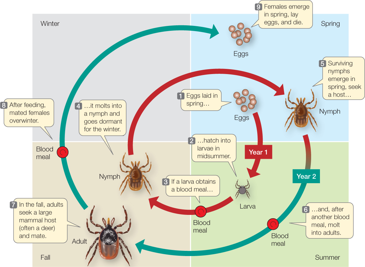
The study of processes that influence birth, death, and population growth rates is known as demography (Greek demos, “population”; graphia, “description”). Ecologists who wish to understand such processes for a species usually begin by characterizing its life history: the sequence of key events, such as growth and development, reproduction, and death, that occur during an average individual’s life. To describe the life history of the black-legged tick, for example, we begin with the first life stage—one of the thousands of eggs laid by an adult female in spring (FIGURE 42.3). If the egg survives, it hatches into a larva in midsummer. If the larva can obtain a blood meal from a mammal, bird, or lizard, it molts into a nymph and goes dormant for the winter. If it survives the winter, the nymph becomes active again the following summer and seeks another blood meal from a vertebrate host. If it is successful, it molts into an adult in the fall and seeks a large mammal host, such as a deer, raccoon, opossum—or human. If successful, it mates on this final host, and if it is a female, goes dormant for another winter, lays eggs in the spring, and dies.
868

Go to MEDIA CLIP 42.1 Dangerous Deer Ticks
PoL2e.com/mc42.1
Even this qualitative description of the tick’s life history gives us important insights into its ecological interactions. But to estimate birth and death rates, we need more information about the timing of life events and the number of offspring produced. A quantitative tick life history would indicate at what ages individuals make transitions between life stages and how many do so successfully: the fraction of eggs that hatch successfully, of larvae that find a host and molt successfully into nymphs, and of nymphs that live through the winter, find a host, and molt into adults. In addition, a quantitative life history would indicate the number of eggs that the average adult female lays.
Obtaining such information is not easy, and ecologists still don’t have all of it for black-legged ticks. We do have quantitative life histories, however, for other species, such as the common cactus finch (Geospiza scandens) in the Galápagos archipelago. TABLE 42.1 shows the life history, in table form, of a sample of 210 finches born on a single island in 1978. The table quantifies two important aspects of any life history: the fraction of individuals that survive from birth to different life stages (which are ages in the case of the finches), called survivorship; and the average number of offspring each surviving individual produces at those life stages, called fecundity. Survivorship can also be expressed as its opposite, mortality, which is the fraction of individuals that do not survive from birth to a given stage or age (mortality = 1 − survivorship).
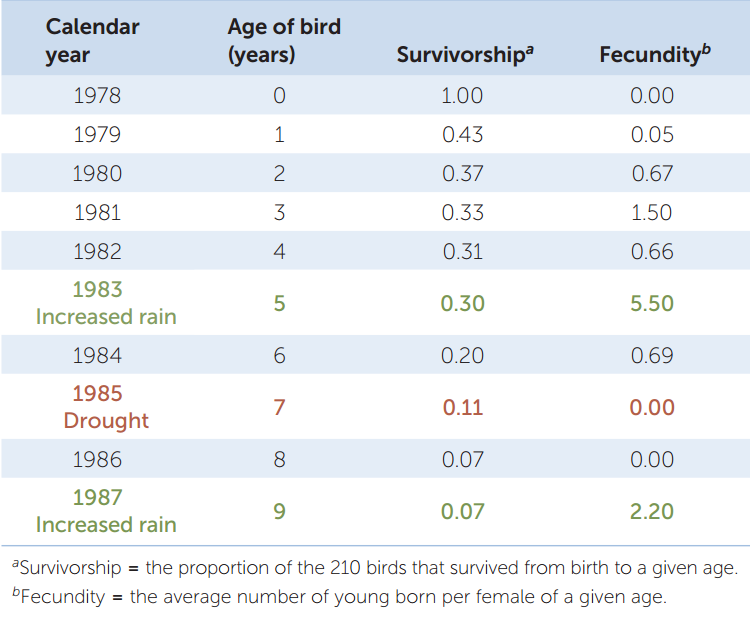
Information on survivorship, fecundity, and the duration of life stages can be used to calculate per capita growth rates (r) for any life history. The calculations involved are complex, but it is not hard to see that survivorship and fecundity will affect r. All else being equal, the higher the fecundity and the higher the survivorship, the higher r will be. If reproduction shifts to earlier ages, r will increase as well.
Life histories are diverse
Species vary considerably in how many and what types of life stages they go through, how old they are when they begin to reproduce, how often they reproduce, how many offspring they produce, and how long they live. Most black-legged ticks spin out their lives over 2 years, whereas the life history of a periodical cicada spans nearly 2 decades. Other arthropods have life spans of days or weeks. Some species, like the tick, go through a discrete series of life stages of variable duration, each separated by a molt. Other species, such as common cactus finches and humans, develop continuously as they age. Some plants germinate, grow, flower, produce seeds, and die all in one growing season—they are annuals (see Concept 27.2). Other plants live for centuries. Some species spend long periods in a dormant state, whereas others are continuously active. Some organisms, including the tick, reproduce only once and then die; others, such as finches and humans, can reproduce multiple times.
869
Life histories vary not only among species but within species as well, including among human populations. For example, life expectancy (the age to which an average person survives) of the Aeta people of the Philippines, who hunt and gather wild food, is 16.5 years, and girls reach puberty at age 12. The Turkana, herders of East Africa, experience food shortages as frequently as the Aeta, but they have a life expectancy of 47.5 years, and Turkana women reach sexual maturity at age 15. In well-nourished United States populations, life expectancy is 78.2 years—much greater than for either the Aeta or the Turkana—yet girls in the U.S. reach puberty at age 12.5 years on average.
Resources and physical conditions shape life histories
Individual organisms must acquire materials and energy to maintain themselves and to fuel metabolism, growth, activity, defense, and reproduction. Materials and energy—and the time available to acquire them—constitute resources for organisms. Organisms also need physical conditions that they are able to tolerate. The primary distinction between resources and conditions is that resources can be used up (e.g., mineral nutrients, photons of light, time, space, or food items), whereas conditions are experienced but not consumed.
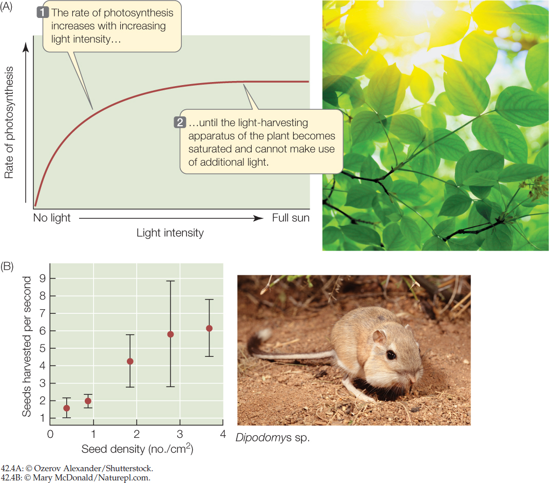
The rate at which an organism can acquire a resource increases with the availability of that resource in its environment, up to the point at which the organism’s capacity to take in and process the resource is saturated. A plant’s net photosynthetic rate, for example, increases with sunlight intensity (FIGURE 42.4A), and an animal’s rate of food intake increases with the density of food (FIGURE 42.4B)—but in both cases we see a leveling off of intake rate at high resource availability.
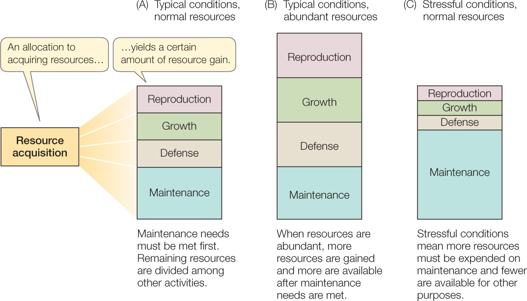
Organisms use the resources they obtain for functions such as maintenance, growth (see Concept 29.1), defense (see Chapter 39), and reproduction (see Chapter 37) (FIGURE 42.5). In addition, they must devote some resources to activities involved in obtaining more resources. The principle of allocation states that once an organism has acquired a unit of some resource (such as food), that bit of resource cannot be used for multiple functions at once.
870
In general, an organism’s first priority is to maintain the integrity of its body. Investment in maintenance is greater in stressful than in unstressful environments because maintenance is more difficult under stressful physical conditions (as was illustrated for temperature in Concept 29.3). For example, the hotter their desert environment, the more time day-active lizards must spend in a cool retreat to keep body temperature below a lethal level, and thus the less time they have to look for food (see Figure 29.8). Once an organism obtains more resources than it needs for maintenance, it can allocate the excess to other functions, such as growing bigger or producing offspring. In general, as the average individual in a population acquires more resources, the average fecundity and survivorship increase.
Life-history variation among species and populations often reflects the principle of allocation. A species that invests heavily in growth early in life, for example, cannot simultaneously invest heavily in defense (e.g., protective structures or chemical defenses). As a consequence, it reaches adult size quickly, but at the cost of lower survivorship than a species that invests more in defense. A species that starts investing in reproduction early in life grows more slowly, and matures at a smaller adult size, than a species that waits to reproduce. Species that invest heavily in reproduction often do so at the expense of adult survivorship. They have high fecundity but short life spans. Such negative relationships among growth, reproduction, and survival are called life-history trade-offs.
The environment shapes much of this life-history variation because, together with a species’ way of life, it determines the relative costs and benefits, in terms of survivorship and fecundity, of any particular allocation pattern. The Aeta people mentioned earlier, for example, live in an environment that imposes higher mortality than does that of the Turkana. High mortality means that the benefit of early reproduction (more individuals survive to reproduce at least once) outweighs the fecundity benefit of growing to a larger adult size (in general, human females produce 0.24 more offspring per additional centimeter of height). Most Aeta women reach puberty and stop growing at about 12 years of age, at an adult height averaging 140 cm. For the Turkana, the lower mortality rate shifts the balance—the advantage of early reproduction is outweighed by the fecundity advantage of attaining a larger adult size. Turkana women mature at age 15 and at a height averaging 166 cm. In the United States, plentiful food and modern medicine reduce the cost of maturing early—girls grow fast and mature early, at an adult size equivalent to that of the Turkana.
In a similar way, the short summers in New York State make it advantageous for black-legged tick nymphs to invest in overwinter survival, even though it means that most individuals do not reproduce until their second year (see Figure 42.3), and a few take even longer. Ticks find their hosts by waiting: they climb up on vegetation, extend their forelegs, and climb aboard when a host bumps into them. Finding a host is such a rare event that a tick can expect at most one meal during the short growing season. As a result, nymphs do not allocate resources to further host-seeking behavior during their first season of life, but instead allocate resources to overwinter survival. The fact that ticks take 2 years to complete their life history is thus a consequence of the difficulty of encountering a host and the seasonality of the environment.
Species’ distributions reflect the effects of environment on per capita growth rates
A population cannot persist in an environment where its per capita growth rate is negative, because its size would inevitably shrink to zero—it would go extinct. We can predict where populations are likely to be found if we know how resource availability and physical conditions affect survivorship and fecundity. Obtaining complete knowledge of life histories is often impossible for species in the wild, but even incomplete knowledge helps us understand species’ distributions. FIGURE 42.6 illustrates this point for the lizard Sceloporus serrifer. By combining measurements of conditions in the lizard’s natural environment with knowledge of its physiology and behavior, researchers were able to draw conclusions about how climate change is affecting the lizard’s survivorship, fecundity, and distribution—with important implications for its conservation.
Investigation
HYPOTHESIS
Spiny lizards have fewer hours to forage on hotter days.
METHOD
- Construct model “lizards” that have the same thermal properties as real lizards.
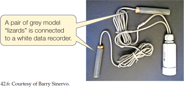 Figure 42.6: Climate Warming Stresses Spiny Lizards Barry Sinervo and colleagues wanted to know whether climate warming will stress Mexican blue spiny lizards (Sceloporus serrifer) by reducing the number of hours they can remain outside their burrows without overheating. These lizards feed only during daytime and retreat to their cool burrows when their body temperature gets too high (see Figure 29.8). In 2008, the researchers conducted experiments in four locations in Mexico where these lizards had been found in 1975. Climate records indicated that the four locations did not warm at the same rate between 1975 and 2008, perhaps because they differ in such things as proximity to the ocean, elevation above sea level, and latitude.a
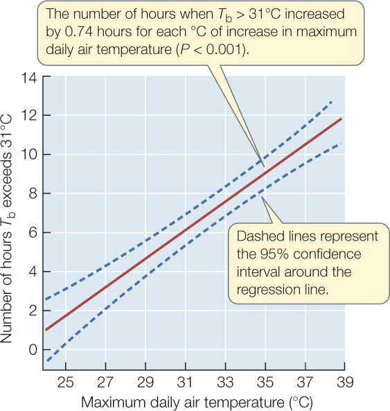
 - At four sites in the Yucatán where lizards occurred in 1975, place replicate model lizards in various perches that real lizards use when they forage. Monitor body temperature Tb of the models each hour and record maximum daily air temperatures during the breeding season (March and April).
- For each day, calculate the number of hours that the body temperature Tb of the model lizards exceeded 31°C—the temperature at which S. serrifer are known to stop foraging and retreat to their burrows—to arrive at a predicted number of inactive hours for real lizards.
- Determine whether the predicted number of inactive hours increased with maximum daily air temperature.
RESULTS
CONCLUSION
The hypothesis is supported by the data: S. serrifer can forage without overheating for fewer hours on days when maximum air temperature is higher.
ANALYZE THE DATA
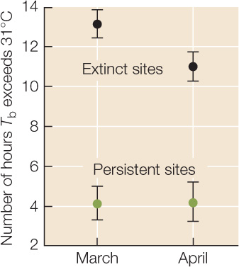
Between 1975 and 2008, S. serrifer populations went extinct at two of the four sites monitored by Sinervo and colleagues. The graph at right shows March and April averages in 2008 for the number of hours (in some cases including hours after sundown!) when Tb > 31°C at the two “extinct” sites and at the two “persistent” sites. Error bars are 1 standard error of the mean (see Appendix B); sample size for each point is 240 observations (2 sites × 30 days × 4 lizard models). Use this graph to answer the questions below.
- How did the hours available for foraging differ between the “extinct” sites (black symbols) and the “persistent” sites (green symbols)?
- How might the availability of foraging time influence lizard fecundity, survivorship, and per capita growth rates?
- Sinervo and colleagues knew that climate warming had taken place between 1975 and 2008 (for example, see Figure 45.13), the period during which some of the lizard populations had gone extinct. Is the extinction of some, but not all, lizard populations consistent with the conclusion that climate warming was one of the causes of extinction? Why or why not?
Go to LaunchPad for discussion and relevant links for all INVESTIGATION figures.
aB. Sinervo et al. 2010. Science 328: 894–899.
871
872
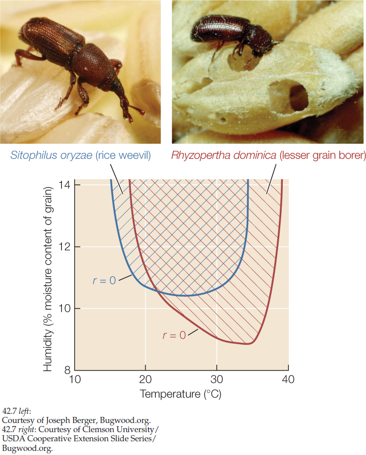
Sometimes it is possible to explore the links between environmental conditions, life histories, and species distributions with the help of experiments carried out in the laboratory. Charles Birch used this approach to understand why two species of beetles that infest stored grain are serious pests in some parts of Australia but not in others. In his laboratory, Birch reared populations of the rice weevil (Sitophilus oryzae, known in Birch’s time as Calandra oryzae) and the lesser grain borer (Rhyzopertha dominica) under various conditions of temperature and humidity. He quantified beetle life histories for each set of conditions and used survivorship and fecundity data to calculate per capita growth rates for each species under those conditions. The results, summarized in FIGURE 42.7, explain the more tropical geographic range of R. dominica. In addition, both species had negative per capita growth rates in cool, dry environments. This finding suggested a strategy for managing stores of grain to minimize losses: keep the grain cool and dry.
CHECKpoint CONCEPT 42.3
- When kangaroo rats harvest seeds, they grab them with their front paws and put them into “grocery bags”—cheek pouches (see Figure 42.4B). Based on the graph in that figure, what do you think the harvest rate would be if seed density increased to 5 seeds/cm2? Explain.
- Female hummingbirds in the Rocky Mountains usually live long enough to reproduce for several summer seasons. If they still have young in the nest when the supply of food (nectar produced by flowers) declines toward zero at the end of the summer, they abandon the nest and the young. Can you explain this behavior in terms of the principle of allocation?
- In an experiment, ecologists added predatory fish to some streams, leaving other streams predator-free as controls. How would you expect size and age of first reproduction of prey fish to evolve in the presence of predators? (Hint: Consider the example of the Aeta and Turkana.)
- Explain how the results shown in Figure 42.7 are consistent with the grain borer Rhyzopertha dominica having a more tropical geographic range than the rice weevil Sitophilus oryzae. (Hint: See Concept 41.2.)
Knowing whether population growth rates are negative or positive in particular environments tells us why species are absent or present in those environments. But this knowledge does not help us understand why population densities vary among different locations where population growth rates are positive. To do so, we must take a closer look at the dynamics of population growth.