11.3 Multiple Regression Model Building
Often, we have many explanatory variables, and our goal is to use these to explain the variation in the response variable. A model using just a few of the variables often predicts about as well as the model using all the explanatory variables. We may also find that the reciprocal of a variable is a better choice than the variable itself or that including the square of an explanatory variable improves prediction. How can we find a good model? That is the model building issue. A complete discussion would be quite lengthy, so we must be content with illustrating some of the basic ideas with a Case Study.
model building
Case 11.3 Prices of Homes

homes
People wanting to buy a home can find information on the Internet about homes for sale in their community. We work with online data for homes for sale in Lafayette and West Lafayette, Indiana.16 The response variable is Price, the asking price of a home. The online data contain the following explanatory variables: (a) SqFt, the number of square feet for the home; (b) BedRooms, the number of bedrooms; (c) Baths, the number of bathrooms; (d) Garage, the number of cars that can fit in the garage; and (e) Zip, the postal zip code for the address. There are 504 homes in the data set.
The analysis starts with a study of the variables involved. Here is a short summary of this work.
567
Price, as we expect, has a right-skewed distribution. The mean (in thousands of dollars) is $158 and the median is $130. There is one high outlier at $830, which we delete as unusual in this location. Remember that a skewed distribution for Price does not itself violate the conditions for multiple regression. The model requires that the residuals from the fitted regression equation be approximately Normal. We have to examine how well this condition is satisfied when we build our regression model.
BedRooms ranges from one to five. The website uses five for all homes with five or more bedrooms. The data contain just one home with one bedroom. Baths includes both full baths (with showers or bathtubs) and half baths (which lack bathing facilities). Typical values are 1, 1.5, 2, and 2.5. Garage has values of 0, 1, 2, and 3. The website uses the value 3 when three or more vehicles can fit in the garage. There are 50 homes that can fit three or more vehicles into their garage (or possibly garages). The data set has begun a process of combining some values of these variables, such as five or more bedrooms and garages that hold three or more vehicles. We continue this process as we build models for predicting Price.
Zip describes location, traditionally the most important explanatory variable for house prices, but Zip is a quite crude description because a single zip code covers a broad area. All of the postal zip codes in this community have 4790 as the first four digits. The fifth digit is coded as the variable Zip. The possible values are 1, 4, 5, 6, and 9. There is only one home with zip code 47901. We first look at the houses in each zip code separately.
SqFt, the number of square feet for the home, is a quantitative variable that we expect to strongly influence Price. We start our analysis by examining the relationship between Price and this explanatory variable. To control for location, we start by examining only the homes in zip code 47904, corresponding to . Most homes for sale in this area are moderately priced.
EXAMPLE 11.17 Price and Square Feet
homes04
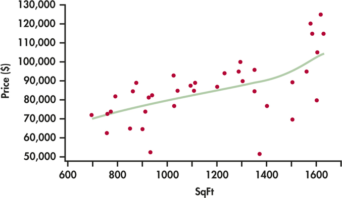
CASE 11.3 The HOMES data set contains 44 homes for sale in zip code 47904. We focus on this subset. Preliminary examination of Price reveals that a few homes have prices that are somewhat high relative to the others. Similarly, some values for SqFt are relatively high. Because we do not want our analysis to be overly influenced by these homes, we exclude any home with Price greater than $150,000 and any home with SqFt greater than 1800 ft2. Seven homes were excluded by these criteria.
Figure 11.13 displays the relationship between SqFt and Price. We have added a "smooth’’ fit to help us see the pattern. The relationship is approximately linear but curves up somewhat for the higher-priced homes.
568
Because the relationship is approximately linear and we expect SqFt to be an important explanatory variable, let’s start by examining the simple linear regression of Price on SqFt.
EXAMPLE 11.18 Regression of Price on Square Feet
homes04
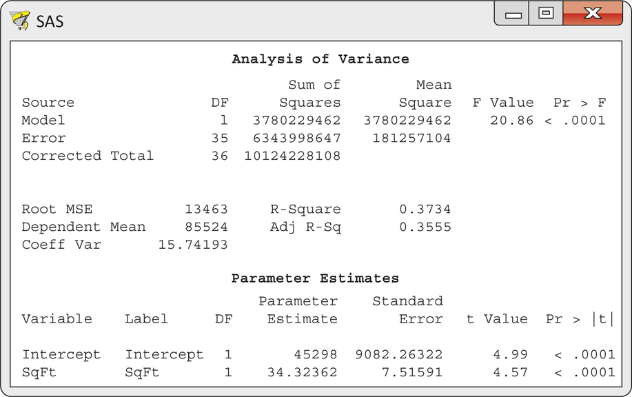
CASE 11.3 Figure 11.14 gives the regression output. The number of degrees of freedom in the "Corrected Total’’ line in the ANOVA table is 36. This is correct for the homes that remain after we excluded seven of the original 44. The fitted model is
The coefficient for SqFt is statistically significant (, , ). Each additional square foot of area raises selling prices by $34.32 on the average. From the , we see that 37.3% of the variation in the home prices is explained by a linear relationship with square feet. We hope that multiple regression will allow us to improve on this first attempt to explain selling price.
Apply Your Knowledge
Question 11.59
11.59 Distributions.
CASE 11.3 Make stemplots or histograms of the prices and of the square feet for the 44 homes in Table 11.6. Do the seven homes excluded in Example 11.17 appear unusual for this location?
11.59
The 7 houses all appear in the tails of the distributions helping to form the right-skew, but they are not outliers.
homes04
Question 11.60
11.60 Plot the residuals.
CASE 11.3 Obtain the residuals from the simple linear regression in the preceding example and plot them versus SqFt. Describe the plot. Does it suggest that the relationship might be curved?
homes04
Question 11.61
11.61 Predicted values.
CASE 11.3 Use the simple linear regression equation to obtain the predicted price for a home that has 1750 ft2. Do the same for a home that has 2250 ft2.
569
| Id | Price ($ thousands) |
SqFt | BedRooms | Baths | Garage | Id | Price ($ thousands) |
SqFt | BedRooms | Baths | Garage |
|---|---|---|---|---|---|---|---|---|---|---|---|
| 01 | 52,900 | 932 | 1 | 1.0 | 0 | 23 | 75,000 | 2188 | 4 | 1.5 | 2 |
| 02 | 62,900 | 760 | 2 | 1.0 | 0 | 24 | 76,900 | 1400 | 3 | 1.5 | 2 |
| 03 | 64,900 | 900 | 2 | 1.0 | 0 | 25 | 81,900 | 796 | 2 | 1.0 | 2 |
| 04 | 69,900 | 1504 | 3 | 1.0 | 0 | 26 | 84,500 | 864 | 2 | 1.0 | 2 |
| 05 | 76,900 | 1030 | 3 | 2.0 | 0 | 27 | 84,900 | 1350 | 3 | 1.0 | 2 |
| 06 | 87,900 | 1092 | 3 | 1.0 | 0 | 28 | 89,600 | 1504 | 3 | 1.0 | 2 |
| 07 | 94,900 | 1288 | 4 | 2.0 | 0 | 29 | 87,000 | 1200 | 2 | 1.0 | 2 |
| 08 | 52,000 | 1370 | 3 | 1.0 | 1 | 30 | 89,000 | 876 | 2 | 1.0 | 2 |
| 09 | 72,500 | 698 | 2 | 1.0 | 1 | 31 | 89,000 | 1112 | 3 | 2.0 | 2 |
| 10 | 72,900 | 766 | 2 | 1.0 | 1 | 32 | 93,900 | 1230 | 3 | 1.5 | 2 |
| 11 | 73,900 | 777 | 2 | 1.0 | 1 | 33 | 96,000 | 1350 | 3 | 1.5 | 2 |
| 12 | 73,900 | 912 | 2 | 1.0 | 1 | 34 | 99,900 | 1292 | 3 | 2.0 | 2 |
| 13 | 81,500 | 925 | 3 | 1.0 | 1 | 35 | 104,900 | 1600 | 3 | 1.5 | 2 |
| 14 | 82,900 | 941 | 2 | 1.0 | 1 | 36 | 114,900 | 1630 | 3 | 1.5 | 2 |
| 15 | 84,900 | 1108 | 3 | 1.5 | 1 | 37 | 124,900 | 1620 | 3 | 2.5 | 2 |
| 16 | 84,900 | 1040 | 2 | 1.0 | 1 | 38 | 124,900 | 1923 | 3 | 3.0 | 2 |
| 17 | 89,900 | 1300 | 3 | 2.0 | 1 | 39 | 129,000 | 2090 | 3 | 1.5 | 2 |
| 18 | 92,800 | 1026 | 3 | 1.0 | 1 | 40 | 173,900 | 1608 | 2 | 2.0 | 2 |
| 19 | 94,900 | 1560 | 3 | 1.0 | 1 | 41 | 179,900 | 2250 | 5 | 2.5 | 2 |
| 20 | 114,900 | 1581 | 3 | 1.5 | 1 | 42 | 199,500 | 1855 | 2 | 2.0 | 2 |
| 21 | 119,900 | 1576 | 3 | 2.5 | 1 | 43 | 80,000 | 1600 | 3 | 1.0 | 3 |
| 22 | 65,000 | 853 | 3 | 1.0 | 2 | 44 | 129,000 | 2296 | 3 | 2.5 | 3 |
11.61
.
homes04
Models for curved relationships
Figure 11.13 suggests that the relationship between SqFt and Price may be slightly curved. One simple kind of curved relationship is a quadratic function. To model a quadratic function with multiple regression, create a new variable that is the square of the explanatory variable and include it in the regression model. There are now explanatory variables, and . The model is
with the usual conditions on the .
EXAMPLE 11.19 Quadratic Regression of Price on Square Feet
homes04
CASE 11.3 To predict price using a quadratic function of square feet, first create a new variable by squaring each value of SqFt. Call this variable SqFt2. Figure 11.15 displays the output for multiple regression of Price on SqFt and SqFt2. The fitted model is
570
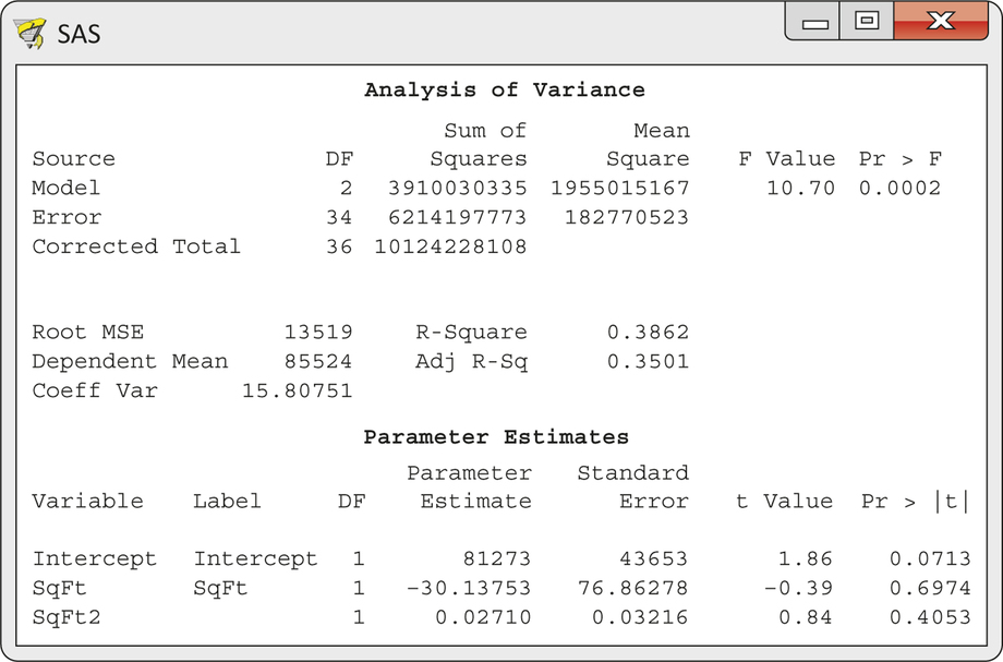
This model explains 38.6% of the variation in Price, little more than the 37.3% explained by simple linear regression of Price on SqFt. The coefficient of SqFt2 is not significant (, , ). That is, the squared term does not significantly improve the fit when the SqFt term is present. We conclude that adding SqFt2 to our model is not helpful.
The output in Figure 11.15 is a good example of the need for care in interpreting multiple regression. The individual tests for both SqFt and SqFt2 are not significant. Yet, the overall test for the null hypothesis that both coefficients are zero is significant (, , ). To resolve this apparent contradiction, remember that a test assesses the contribution of a single variable, given that the other variables are present in the model. Once either SqFt or SqFt2 is present, the other contributes very little. This is a consequence of the fact that these two variables are highly correlated. This phenomenon is called collinearity or multicollinearity. In extreme cases, collinearity can cause numerical instabilities, and the results of the regression calculations can become very imprecise. Collinearity can exist between seemingly unrelated variables and can be hard to detect in models with many explanatory variables. Some statistical software packages will calculate a variance inflation factor (VIF) value for each explanatory variable in a model. VIF values greater than 10 are generally considered an indication that severe collinearity exists among the explanatory variables in a model. Exercise 11.80 (page 583) explores the calculation and use of VIF values. In this particular case, we could dispense with either SqFt or SqFt2, but the test tells us that we cannot drop both of them. It is natural to keep SqFt and drop its square, SqFt2.
collinearity multicollinearity
variance inflation factor (VIF)
Multiple regression can fit a polynomial model of any degree:
In general, we include all powers up to the highest power in the model. A relationship that curves first up and then down, for example, might be described by a cubic model with explanatory variables , , and . Other transformations of the explanatory variable, such as the square root and the logarithm, can also be used to model curved relationships.
571
Apply Your Knowledge
Question 11.62
11.62 The relationship between SqFt and SqFt2.
CASE 11.3 Using the data set for Example 11.19, plot SqFt2 versus SqFt. Describe the relationship. We know that it is not linear, but is it approximately linear? What is the correlation between SqFt and SqFt2? The plot and correlation demonstrate that these variables are collinear and explain why neither of them contributes much to a multiple regression once the other is present.
homes04
Question 11.63
11.63 Predicted values.
CASE 11.3 Use the quadratic regression equation in Example 11.19 to predict the price of a home that has 1750 ft2. Do the same for a home that has 2250 ft2. Compare these predictions with the ones from an analysis that uses only SqFt as an explanatory variable.
11.63
.
homes04
Models with categorical explanatory variables
Although adding the square of SqFt failed to improve our model significantly, Figure 11.13 (page 567) does suggest that the price rises a bit more steeply for larger homes. Perhaps some of these homes have other desirable characteristics that increase the price. Let’s examine another explanatory variable.
EXAMPLE 11.20 Price and the Number of Bedrooms
homes04
CASE 11.3 Figure 11.16 gives a plot of Price versus BedRooms. We see that there appears to be a curved relationship. However, all but two of the homes have either two or three bedrooms. One home has one bedroom and another has four. These two cases are why the relationship appears to be curved. To avoid this situation, we group the four-bedroom home with those that have three bedrooms () and the one-bedroom home with the homes that have two bedrooms.
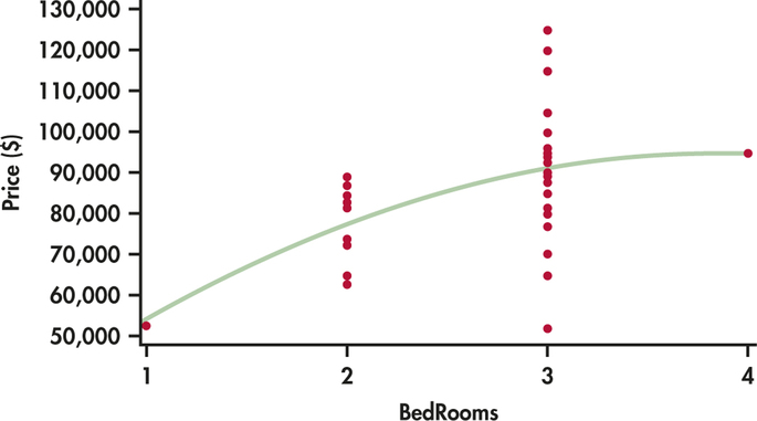
The price of the four-bedroom home is in the middle of the distribution of the prices for the three-bedroom homes. On the other hand, the one-bedroom home has the lowest price of all the homes in the data set. This observation may require special attention later.
"Number of bedrooms’’ is now a categorical variable that places homes in two groups: one/two bedrooms and three/four bedrooms. Software often allows you to simply declare that a variable is categorical. Then the values for the two groups don’t matter. We could use the values 2 and 3 for the two groups. If you work directly with the variable, however, it is better to indicate whether or not the home has three or more bedrooms. We will take the "number of bedrooms’’ categorical variable to be if the home has three or more bedrooms and if it does not. Bed3 is called an indicator variable.
572
Indicator Variables
An indicator variable is a variable with the values 0 and 1. To use a categorical variable that has possible values in a multiple regression, create indicator variables to use as the explanatory variables. This can be done in many different ways. Here is one common choice:
We need only variables to code different values because the last value is identified by "all indicator variables are 0.’’
EXAMPLE 11.21 Price and the Number of Bedrooms
homes04
CASE 11.3 Figure 11.17 displays the output for the regression of Price on the indicator variable Bed3. This model explains 19% of the variation in price. This is about one-half of the 37.3% explained by SqFt, but it suggests that Bed3 may be a useful explanatory variable. The fitted equation is
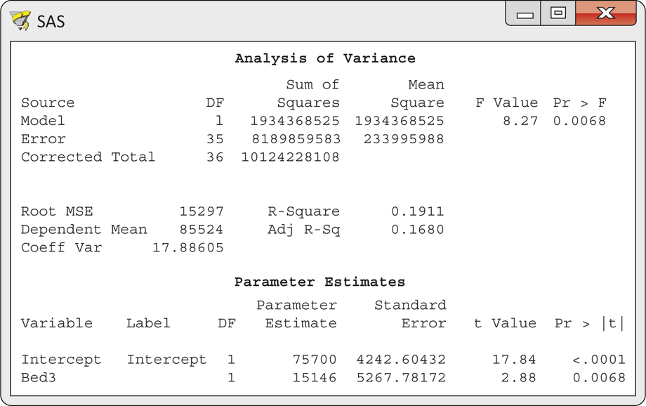
573
The coefficient for Bed3 is significantly different from 0 (, , ). This coefficient is the slope of the least-squares line. That is, it is the increase in the average price when Bed3 increases by 1. The indicator variable Bed3 has only two values, so we can clarify the interpretation.
The predicted price for homes with two or fewer bedrooms () is
That is, the intercept 75,700 is the mean price for homes with . The predicted price for homes with three or more bedrooms () is
That is, the slope 15,146 says that homes with three or more bedrooms are priced $15,146 higher on the average than homes with two or fewer bedrooms. When we regress on a single indicator variable, both intercept and slope have simple interpretations.
Example 11.21 shows that regression on one indicator variable essentially models the means of the two groups. A regression model for a categorical variable with possible values requires indicator variables and therefore regression coefficients (including the intercept) to model the category means. Indicator variables can also be used in models with other variables to allow for different regression lines for different groups. Exercise 11.76 (page 582) explores the use of an indicator variable in a model with another quantitative variable for this purpose.
Here is an example of a categorical explanatory variable with four possible values.
EXAMPLE 11.22 Price and the Number of Bathrooms
homes04
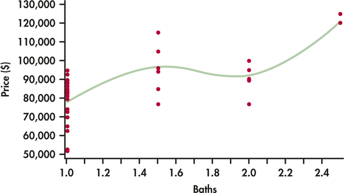
CASE 11.3 The homes in our data set have 1, 1.5, 2, or 2.5 bathrooms. Figure 11.18 gives a plot of price versus the number of bathrooms with a "smooth’’ fit. The relationship does not appear to be linear, so we start by treating the number of bathrooms as a categorical variable. We require three indicator variables for the four values. To use the homes that have one bath as the basis for comparisons, we let this correspond to "all indicator variables equal to 0.’’ The indicator variables are
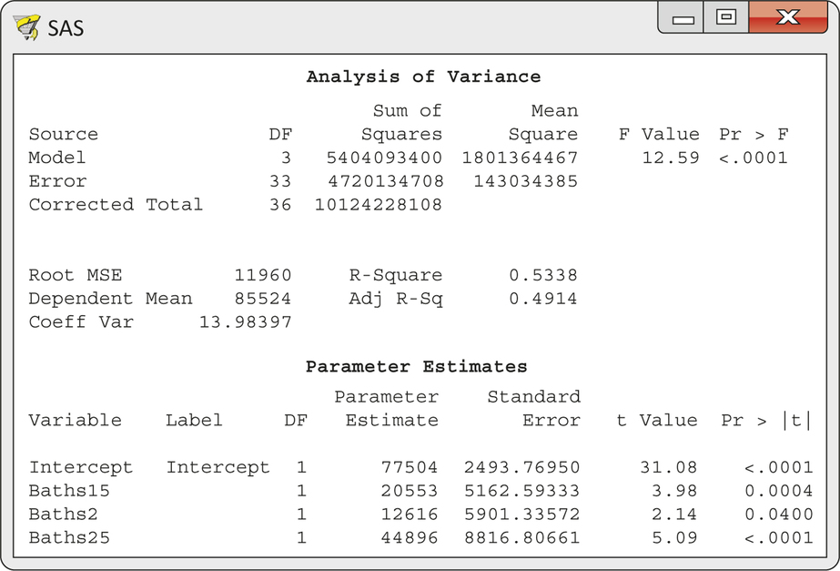
Multiple regression using these three explanatory variables gives the output in Figure 11.19. The overall model is statistically significant (, , ), and it explains 53.3% of the variation in price. This is somewhat more than the 37.3% explained by square feet.
The fitted model is
The coefficients of all the indicator variables are statistically significant, indicating that each additional bathroom is associated with higher prices.
574
Apply Your Knowledge
Question 11.64
11.64 Find the means.
CASE 11.3 Using the data set for Example 11.21, find the mean price for the homes that have three or more bedrooms and the mean price for those that do not.
- Compare these sample means with the predicted values given in Example 11.21.
- What is the difference between the mean price of the homes in the sample that have three or more bedrooms and the mean price of those that do not? Verify that this difference is the coefficient for the indicator variable Bed3 in the regression in Example 11.21.
homes04
Question 11.65
11.65 Compare the means.
CASE 11.3 Regression on a single indicator variable compares the mean responses in two groups. It is, in fact, equivalent to the pooled test for comparing two means (Chapter 7, page 389). Use the pooled test to compare the mean price of the homes that have three or more bedrooms with the mean price of those that do not. Verify that the test statistic, degrees of freedom, and -value agree with the test for the coefficient of Bed3 in Example 11.21.
11.65
.
homes04
575
Question 11.66
11.66 Modeling the means.
CASE 11.3 Following the pattern in Example 11.21, use the output in Figure 11.19 to write the equations for the predicted mean price for the following:
- Homes with 1 bathroom.
- Homes with 1.5 bathrooms.
- Homes with 2 bathrooms.
- Homes with 2.5 bathrooms.
- How can we interpret the coefficient for one of the indicator variables, say Baths2, in language understandable to house shoppers?
More elaborate models
We now suspect that a model that uses square feet, number of bedrooms, and number of bathrooms may explain price reasonably well. Before examining such a model, we use an insight based on careful data analysis to improve the treatment of number of baths.
Figure 11.18 reminds us that the data describe only two homes with 2.5 bathrooms. Our model with three indicator variables fits a mean for these two observations. The pattern of Figure 11.18 reveals an interesting feature: adding a half bath to either one or two baths raises the predicted price by a similar, quite substantial amount. If we use this information to construct a model, we can avoid the problem of fitting one parameter to just two houses.
EXAMPLE 11.23 An Alternative Bath Model
homes04
CASE 11.3 Starting again with one-bath homes as the base (all indicator variables 0), let B2 be an indicator variable for an extra full bath and let Bh be an indicator variable for an extra half bath. Thus, a home with two baths has and . A home with 2.5 baths has and . Regressing Price on Bh and B2 gives the output in Figure 11.20.
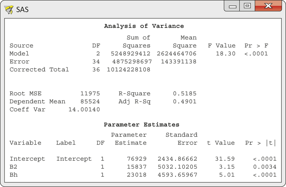
The overall model is statistically significant (, , ), and it explains 51.9% of the variation in price. This compares favorably with the 53.3% explained by the model with three indicator variables for bathrooms. The fitted model is
576
That is, an extra full bath adds $15,837 to the mean price and an extra half bath adds $23,018. The statistics show that both regression coefficients are significantly different from zero (, , ; and , , ).
So far we have learned that the price of a home is related to the number of square feet, whether or not there are three or more bedrooms, whether or not there is an additional full bathroom, and whether or not there is an additional half bathroom. Let’s try a model including all these explanatory variables.
EXAMPLE 11.24 Square Feet, Bedrooms, and Bathrooms
homes04
CASE 11.3 Figure 11.21 gives the output for predicting price using SqFt, Bed3, B2, and Bh. The overall model is statistically significant (, , ), and it explains 58.9% of the variation in price.
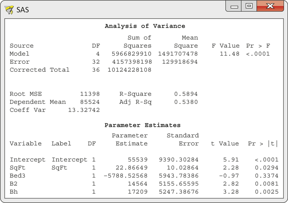
The individual for Bed3 is not statistically significant (, , ). That is, in a model that contains square feet and information about the bathrooms, there is no additional information in the number of bedrooms that is useful for predicting price. This happens because the explanatory variables are related to each other: houses with more bedrooms tend to also have more square feet and more baths.
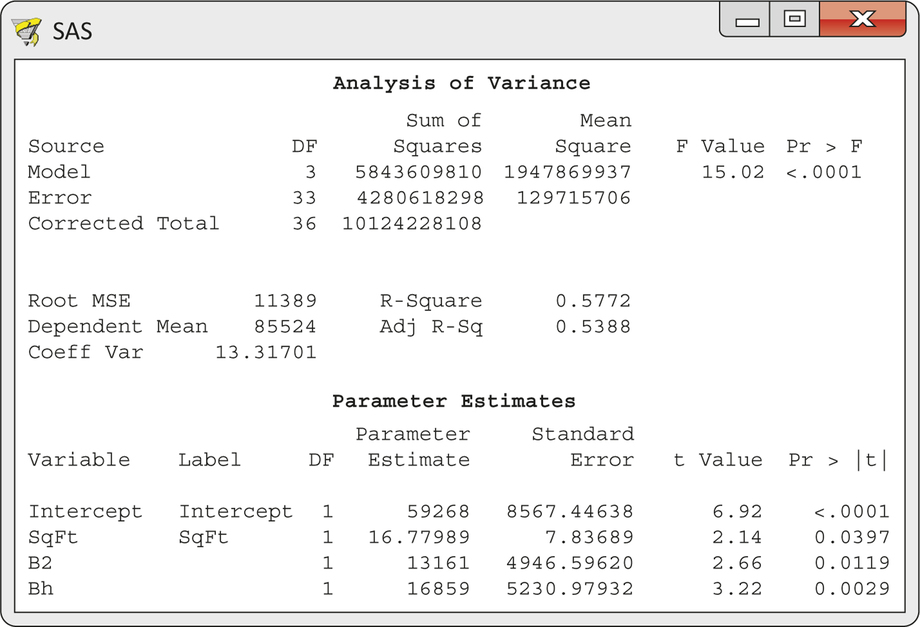
Therefore, we redo the regression without Bed3. The output appears in Figure 11.22. The value of has decreased slightly to 57.7%, but now all the coefficients for the explanatory variables are statistically significant. The fitted regression equation is
577
Apply Your Knowledge
Question 11.67
11.67 What about garages?
CASE 11.3 We have not yet examined the number of garage spaces as a possible explanatory variable for price. Make a scatterplot of price versus garage spaces. Describe the pattern. Use a "smooth’’ fit if your software has this capability. Otherwise, find the mean price for each possible value of Garage, plot the means on your scatterplot, and connect the means with lines. Is the relationship approximately linear?
11.67
Other than the 1 house with 3 garage spaces, the plot is quite linear between 0 and 2 spaces.
homes04
Question 11.68
11.68 The home with three garages.
CASE 11.3 There is only one home with three garage spaces. We might either place this house in the group or remove it as unusual. Either decision leaves Garage with values 0, 1, and 2. Based on your plot in the previous exercise, which choice do you recommend?
Variable selection methods
We have arrived at a reasonably satisfactory model for predicting the asking price of houses. But it is clear that there are many other models we might consider. We have not used the Garage variable, for example. What is more, the explanatory variables can interact with each other. This means that the effect of one explanatory variable depends upon the value of another explanatory variable. We account for this situation in a regression model by including interaction terms.
interaction terms
The simplest way to construct an interaction term is to multiply the two explanatory variables together. Thus, if we wanted to allow the effect of an additional half bath to depend upon whether or not there is an additional full bath, we would create a new explanatory variable by taking the product . Interaction terms that are the product of an indicator variable and another variable in the model can be used to allow for different slopes for different groups. Exercise 11.76 (page 582) explores the use of such an interaction term in a model.
578
Considering interactions increases the number of possible explanatory variables. If we start with the five explanatory variables SqFt, Bed3, B2, Bh, and Garage, there are 10 interactions between pairs of variables. That is, there are now 15 possible explanatory variables in all. From 15 explanatory variables, it is possible to build 32,767 different models for predicting price. We need to automate the process of examining possible models.
Modern regression software offers variable selection methods that examine all possible multiple regression models. The software then presents us a list of the top models based on some selection criteria. Available criteria include , the regression standard error s, AIC, and BIC. These latter three criteria balance fit against model simplicity in different ways and are appropriate for comparing models with different numbers of explanatory variables. should only be used when comparing two models with the same number of explanatory variables.
EXAMPLE 11.25 Predicting Asking Price
homes04
CASE 11.3 Software tells us that the highest available increases as we increase the number of explanatory variables as follows:
| Variables | |
|---|---|
| 1 | 0.44 |
| 2 | 0.57 |
| 3 | 0.62 |
| 4 | 0.66 |
| 5 | 0.72 |
| ⋮ | |
| 13 | 0.77 |
Because of collinearity problems, models with 14 or all 15 explanatory variables cannot be used. The highest possible is 77%, using 13 explanatory variables.
There are only 37 houses in the data set. A model with too many explanatory variables will fit the accidental wiggles in the prices of these specific houses and may do a poor job of predicting prices for other houses. This is called overfitting.
overfitting
There is no formula for choosing the "best’’ multiple regression model. We tend to prefer smaller models to larger models because they avoid overfitting. However, too small a model may not fit the data or predict well. Model selection criteria such as the regression standard error or AIC balance these two goals but in different ways. Using one of these is preferred to when trying to determine a best model because does not account for overfitting.
We also want a model that makes intuitive sense. For example, the best single predictor () is SqFtBh, the interaction between square feet and having an extra half bath. In general, we would not use a model that has interaction terms unless the explanatory variables involved in the interaction are also included. The variable selection output does suggest that we include SqFtBh and, therefore, SqFt and Bh.
EXAMPLE 11.26 One More Model
homes04
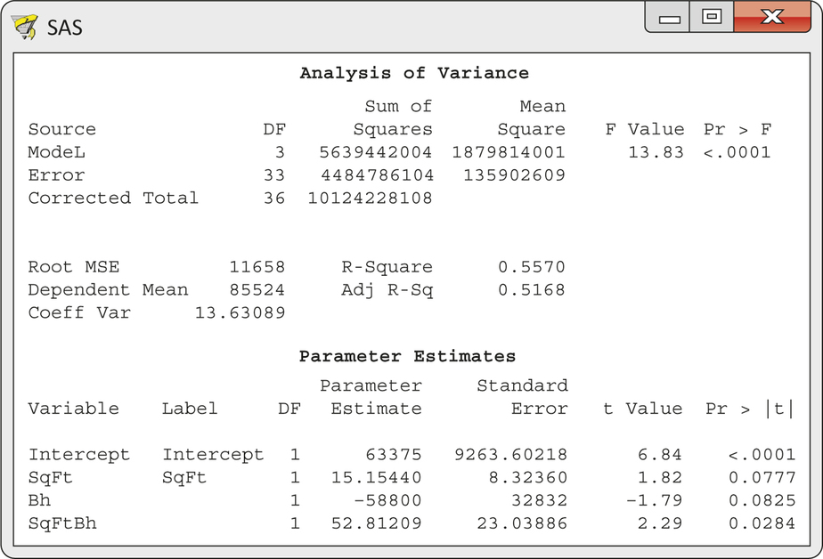
CASE 11.3 Figure 11.23 gives the output for the multiple regression of Price on SqFt, Bh, and the interaction between these variables. This model explains 55.7% of the variation in price. The coefficients for SqFt and Bh are significant at the 10% level but not at the 5% level (, , ; and , , ). However, the interaction is significantly different from zero (, , ). Because the interaction is significant, we keep the terms SqFt and Bh in the model even though their -values do not quite pass the 0.05 standard. The fitted regression equation is
579
The negative coefficient for Bh seems odd. We expect an extra half bath to increase price. A plot will help us to understand what this model says about the prices of homes.
EXAMPLE 11.27 Interpretation of the Fit
homes04
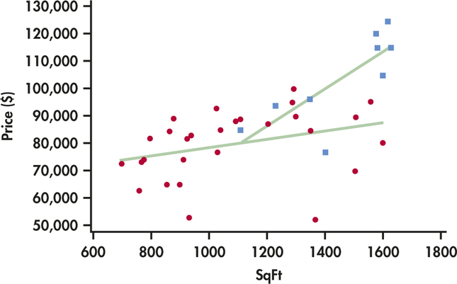
CASE 11.3 Figure 11.24 plots Price against SqFt, using different plot symbols to show the values of the categorical variable Bh. Homes without an extra half bath are plotted as circles, and homes with an extra half bath are plotted as squares. Look carefully: none of the smaller homes have an extra half bath.
580
The lines on the plot graph the model from Example 11.26. The presence of the categorical variable Bh and the interaction account for the two lines. That is, the model expresses the fact that the relationship between price and square feet depends on whether or not there is an additional half bath.
We can determine the equations of the two lines from the fitted regression equation. Homes that lack an extra half bath have . When we set in the regression equation
we get
For homes that have an extra half bath, and the regression equation becomes
In Figure 11.24, we graphed this line starting at the price of the least-expensive home with an extra half bath. These two equations tell us that an additional square foot increases asking price by $15.15 for homes without an extra half bath and by $67.96 for homes that do have an extra half bath.
Apply Your Knowledge
Question 11.69
11.69 Comparing some predicted values.
CASE 11.3 Consider two homes, both with 2000 ft2. Suppose the first has an extra half bath and the second does not. Find the predicted price for each home and then find the difference.
11.69
For the home with the extra half bath, .For the home without, . The difference is $46,820.
Question 11.70
11.70 Suppose the homes are larger.
CASE 11.3 Consider two additional homes, both with 2500 ft2, one with an extra half bath and one without. Find the predicted prices and the difference. How does this difference compare with the difference you obtained in the previous exercise? Explain what you have found.
Question 11.71
11.71 How about the smaller homes?
CASE 11.3 Would it make sense to do the same calculations as in the previous two exercises for homes that have 700 ft2? Explain why or why not.
11.71
No, it would not make sense. As we saw in the interaction plot, homes less than 1000 square feet don’t have an extra half bath.
Question 11.72
11.72 Residuals.
CASE 11.3 Once we have chosen a model, we must examine the residuals for violations of the conditions of the multiple regression model. Examine the residuals from the model in Example 11.26.
- Plot the residuals against SqFt. Do the residuals show a random scatter, or is there some systematic pattern?
- The residual plot shows three somewhat low residuals, between −$20,000 and −$40,000. Which homes are these? Is there anything unusual about these homes?
- Make a Normal quantile plot of the residuals. (Make a histogram if your software does not make Normal quantile plots.) Is the distribution roughly Normal?
homes04
BEYOND THE BASICS: Multiple Logistic Regression
Many studies have yes/no or success/failure response variables. A surgery patient lives or dies; a consumer does or does not purchase a product after viewing an advertisement. Because the response variable in a multiple regression is assumed to have a Normal distribution, this methodology is not suitable for predicting yes/no responses. However, there are models that apply the ideas of regression to response variables with only two possible outcomes.
581
logistic regression
The most common technique is called logistic regression, which we discuss in Chapter 17. The starting point is that if each response is 0 or 1 (for failure or success), then the mean response is the probability of a success. Logistic regression tries to explain in terms of one or more explanatory variables. Details are even more complicated than those for multiple regression, but the fundamental ideas are very much the same and software handles most details. Here is an example.
EXAMPLE 11.28 Sexual Imagery in Advertisements
Marketers sometimes use sexual imagery in advertisements targeted at teens and young adults. One study designed to examine this issue analyzed how models were dressed in 1509 ads in magazines read by young and mature adults.17 The clothing of the models in the ads was classified as not sexual or sexual. Logistic regression was used to model the probability that the model’s clothing was sexual as a function of four explanatory variables.18 Here, model clothing with values 1 for sexual and 0 for not sexual is the response variable.
The explanatory variables were , a variable having the value 1 if the median age of the readers of the magazine is 20 to 29 and 0 if the median age of the readers of the magazine is 40 to 49; , the gender of the model, coded as 1 for female and 0 for male; , a code to indicate men’s magazines, with values 1 for a men’s magazine and 0 otherwise; and , a code to indicate women’s magazines, with values 1 for a women’s magazine and 0 otherwise. General-interest magazines are coded as 0 for both and .
The fitted model is
Interpretation of the coefficients is a little more difficult in multiple logistic regression because of the form of the model. The expression is the odds that the model is sexually dressed. Logistic regression models the "log odds’’ as a linear combination of the explanatory variables. Positive coefficients are associated with a higher probability that the model is dressed sexually. We see that ads in magazines with younger readers, female models, and women’s magazines are more likely to show models dressed sexually.
odds
Similar to the test in multiple regression, there is a chi-square test for multiple logistic regression that tests the null hypothesis that all coefficients of the explanatory variables are zero. The value is , and the degrees of freedom are the number of explanatory variables, four in this case. The -value is reported as . (You can verify that it is less than 0.0005 using Table F.) We conclude that not all the explanatory variables have zero coefficients.
In place of the tests for individual coefficients in multiple regression, chi-square tests, each with one degree of freedom, are used to test whether individual coefficients are zero. For reader age and model gender, , while for the indicator for women’s magazines, . The indicator for men’s magazines is not statistically significant.