13.4 Lag Regression Models
The previous section applied regression methods from Chapters 10 and 11 to time series data. A time period variable and/or seasonal indicator variables were used as the explanatory variables, and the time series was the response variable. If such explanatory variables are sufficient in modeling the patterns in the time series, then the residuals will be consistent with a random process. As we saw for the Amazon sales series in Example 13.19 (page 678), residuals can still exhibit nonrandom-ness, even after trend and seasonal components are incorporated in the model. Our analysis suggested that we might consider past values of the time series as an explanatory variable.
Lag Variable
A lag variable is a variable based on the past values of the time series.
Recall that we introduced the idea of a lag variable in our development of the ACF. Notationally, if represents the time series in question, then lag variables are given by where is called a lag one variable, is called a lag two variable and so on. Lag variables can be added to the regression model as explanatory variables. The regression coefficients for the lag variables represent multiples of past values for the prediction of future values.
Autoregressive-based models
Can yesterday’s stock price help predict today’s stock price? Can last quarter’s sales be used to predict this quarter’s sales? Sometimes, the best explanatory variables are simply past values of the response variable. Autoregressive time series models take advantage of the linear relationship between successive values of a time series to predict future values of the series.
682
First-Order Autoregressive Model
A first-order autoregressive model specifies a linear relationship between successive values of the time series. The shorthand for this model is AR(1), and the equation is
The preceding model can be expanded to include more lag terms. For example, a time series that is dependent on lag one and lag two variables is referred to as an AR(2) model. Autoregressive models are part of a special class of time series models known as autoregressive integrated moving-average (ARIMA) models (also known as Box-Jenkins models).21 ARIMA model building strives to find the most compact model for the data. For example, in situations in which the modeling of a time series requires the use of many lag variables, the ARIMA model-building strategy would attempt to find an alternative model based on fewer explanatory variables. The approach is beyond the scope of this textbook. Without denying the usefulness of the ARIMA approach, it is reassuring that regression-based modeling is an effective approach for modeling many time series in practice.
EXAMPLE 13.20 Daily Trading Volume of FedEx
fedex
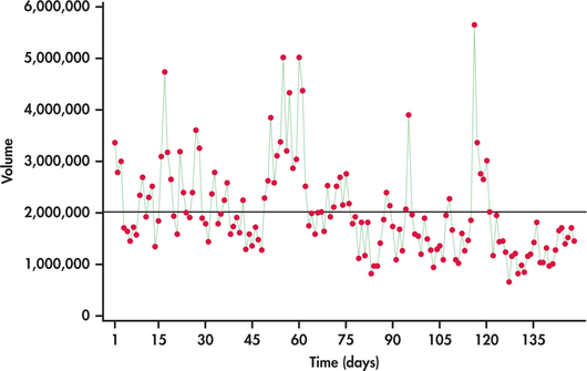
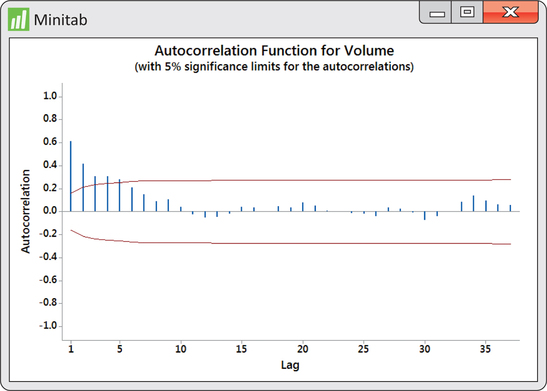
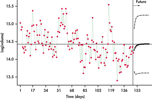
Investors and stock analysts are continually seeking ways to understand price movements in stocks. One factor many have considered in the prediction of price movements is trading volume—that is, the quantity of shares that change owners. In studying the relationship between trading volumes and price movements, an understanding of the trading-volume process becomes a source of interest. Are trading volumes random from trading period to trading period? Or is there some pattern in the trading volumes over time? Figure 13.35 is a time plot of daily trading volumes for FedEx stock from January 2 to August 4, 2014, with the mean trading volume indicated. It appears that there are “strings” of observations either all below or all above the mean. With these strings, we see that if an observation is below (above) the mean, then the next observation quite often will also be below (above) the mean. The ACF of the volumes shown in Figure 13.36 confirms that the series exhibits nonrandom behavior.
683
Notice from Figure 13.35 that the more extreme volumes pull in one direction, namely, upward. If we were to continue our analysis on the volumes, we would find the distribution of residuals to be right-skewed. This situation is similar to the situation of Case 10.1, in which we needed to take the log transformation of income due to its skewness (pages 485–486). We do the same with volumes and transform them with the natural log.
In pursuing the use of lag variables as predictor variables, the natural question is how many lag variables should we use? Looking at the ACF in Figure 13.36, we see that the first five autocorrelations are significant. Does that imply we should entertain a multiple regression on five lag variables? Imagine that there is a strong positive lag one autocorrelation. This would result in adjacent observations being close to each other. In turn, observations two periods apart will also tend to be close to each other, resulting in a positive lag two autocorrelation. So, the lag two autocorrelation is reflecting the effects of the lag one autocorrelation. What we need to know is the correlation between observations two apart after we have adjusted for the effects of the lag one autocorrelation. Similarly, we would want the correlation between observations three apart after we have adjusted for the effects of the lag one and lag two autocorrelations. Such an adjusted correlation is known as partial autocorrelation. Akin to the ACF, a plot of the partial autocorrelations against the lag is called a partial autocorrelation function (PACF).
partial autocorrelation
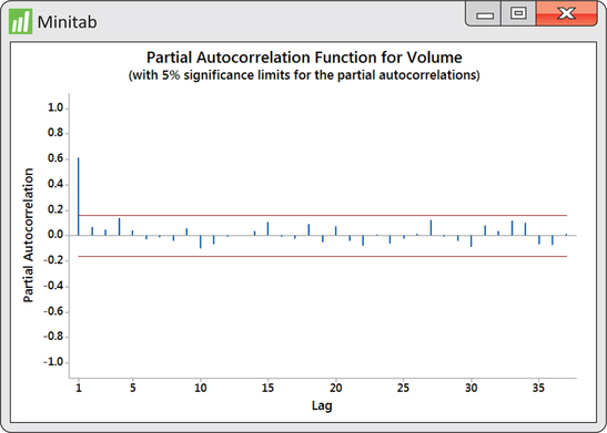
In Figure 13.37, we find the PACF for the logged volumes. Like the ACF, the PACF superimposes significance limits based on 5% level of significance. What we find from the PACF is that we need only consider a lag one variable for our model building. In other words, we pursue the fitting of an AR(1) model.
684
EXAMPLE 13.21 Fitting FedEx Trading Volumes
fedex
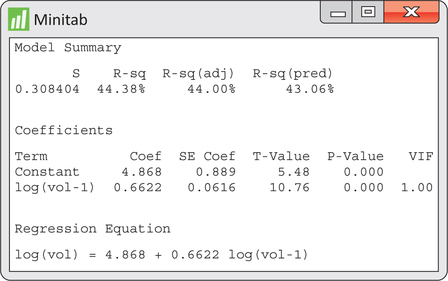
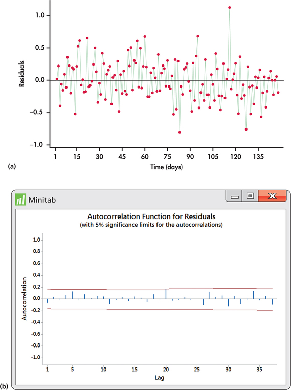
Figure 13.38 displays regression output for the estimated AR(1) fitted model of logged volumes. In summary, the fitted model is given by
To check the adequacy of the AR(1) fitted model, we turn our attention to the time plot of residuals in Figure 13.39(a). The residuals show a mix of short runs and some oscillation with no strong tendency toward one or the other behavior. The ACF of residuals shown in Figure 13.39(b) confirm that the residuals are indeed consistent with randomness.
685
The log volume series ends with , which is slightly less than the overall mean of 14.4292. The forecast for the next day log volume is
Notice that the forecast of 14.2599 is slightly greater than the observed value of 14.1829. The forecast reflects the tendency of the series to revert back to the overall mean.
Our forecast of the next day’s log volume was based on an observed data value—today’s log volume, which is a known value in our time series. If we wish to forecast two days into the future, we have to base our forecast on an estimated value because the next day’s value is not a known value in our time series.
686
EXAMPLE 13.22 Forecasting Two Periods Ahead
Because our time series ends with log(), the value of log() is not known. In its place, we will use the value of calculated in Example 13.21:
The forecast two periods into the future shows further reversion back to the overall mean.
Example 13.21 illustrated a one-step ahead forecast, while Example 13.22 illustrated a two-step ahead forecast. The process shown in Example 13.22 can be repeated to produce forecasts even further into the future.
one-step ahead forecast
In Chapters 10 and 11, we calculated prediction intervals for the response in our regression model. The regression procedures of these chapters can be used to construct prediction intervals for one-step ahead forecasts based on an AR(1) model fit. A difficulty arises when seeking two-step ahead or more prediction intervals. The one-step ahead forecast depends on our estimated values of and and the known value of log(). However, our forecast of log() depends on estimated values of , and log(). The additional uncertainty involved in estimating log() makes the two-ahead prediction interval wider than the one-step ahead prediction interval.
Standard regression procedures do not incorporate the extra uncertainty associated with using estimates of future values in the regression model. In this situation, you want to use time series routines in statistical software to calculate the appropriate prediction intervals. Using Minitab’s AR(1) model-fitting routine, Figure 13.40 displays forecasts along with prediction limits for several years into the future. Notice that the forecasts converge to the overall mean line. Also, the width of the prediction interval initially increases with the first few forecasts and stabilizes moving further into the future.
687
EXAMPLE 13.23 Great Lakes water Levels
lakes
The water levels of the Great Lakes have received much attention in the media. As the world’s largest single source of freshwater, more than 40 million people in the United States and Canada depend on the lakes for drinking water. Economies that greatly depend on the lakes include agriculture, shipping, hydroelectric power, fishing, recreation, and water-intensive industries such as steel making and paper and pulp production.
In the early 1990s, there was a concern that the water levels were too high with the risk to damage shoreline properties. The fear that the lake would engulf shoreline properties was so high that cities like Chicago considered building protection systems that would have cost billions of dollars. Then in the first decade of the twenty-first century, there were great concerns about the water levels being lower than historical averages! The lower levels caused wetlands along the shores to dry up, which could have serious impacts on the reproductive cycle of numerous fish species and ultimately on the fishing industry. The shipping and steel industries were also feeling the effects in that freighters have to carry lighter loads to avoid running aground in shallower harbors.
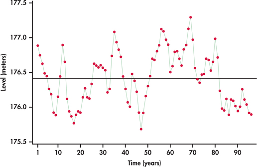
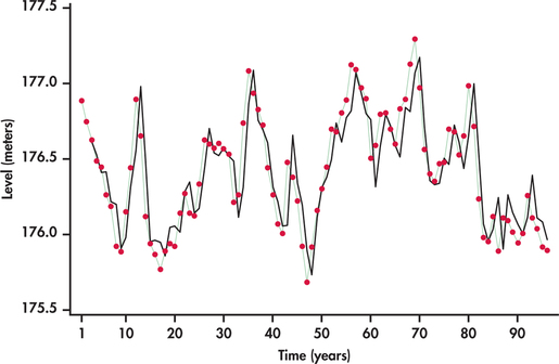
Figure 13.41 displays the average annual water levels (in meters) of Lakes Michigan and Huron from 1918 through 2013.22 We see that the lake levels meander about the mean level. Each time the series drifts away from the overall mean level (above or below), it reverts back toward the mean. There does not seem to be any strong evidence for a long-term trend.
Given the meandering behavior of the lake levels with no obvious trending, the series seems to be a good candidate for modeling with lag variables only.
EXAMPLE 13.24 Fitting Lake Levels
lakes
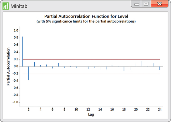
To determine how many lags we should introduce to the model, we obtain the PACF shown in Figure 13.42. The PACF shows that both lag one and lag two correlations are significant. As such, we create a lag one and lag two variable to estimate an AR(2) model. We find the following estimated model:
688
The residuals from this fit show random behavior, indicating that the AR(2) is a good model for the data. Figure 13.43 shows that the AR(2) model does a nice job tracking the water levels over time.
The FedEx and Great Lakes applications gave us opportunities to model series influenced only by autoregressive effects, one as an AR(1) model and the other as an AR(2) model. These autoregressive models are based exclusively on lag variables as predictor variables. In some cases, we need to include lag variables along with other predictor variables to capture the systematic effects.
EXAMPLE 13.25 Fitting and Forecasting Amazon Sales
amazon
CASE 13.1 Example 13.19 (page 678) showed us that the trend-and-season model given in Example 13.18 (pages 675–676) fails to capture the autocorrelation effect between successive observations. One strategy is to add a lag variable to the trend-and-seasonal model. In other words, we need to consider a model for logged sales that combines all the effects:
689
From software, we find the estimated model to be
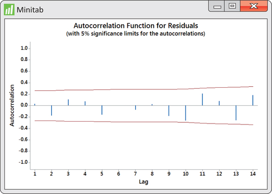
Figure 13.44 shows the ACF for the residuals from the above fit. Compare this ACF with the trend-and-seasonal residuals ACF of Figure 13.34 (page 678). We can see that the lag effects have been captured and thus result in a better fitting model. In terms of forecasting, the series ends with second-quarter 2014 sales of $19,340 (in millions). The ending quarter is the 58th period in the series, so our notation is .
First, use the model to forecast the logarithm of third-quarter 2014 sales:
We can now untransform the log predicted value:
Recall from the discussion of Example 13.18 (pages 675–676) that the preceding fitted value provides a prediction of median sales. If we want a prediction of mean sales, we need to obtain the regression standard error from our log fit. From the regression output for the fitting of logged sales, we find . The predicted mean sales is then
690
In Example 13.18 (pages 675–676), the exponential trend-and-season model predicted sales to be $21.332 billion. Our inclusion of the lag one term in the model adjusted the forecast down by $246 million.
Apply Your Knowledge
Question 13.38
13.38 Unemployment rate.
The Bureau of Labor Statistics tracks national unemployment rates on a monthly and annual basis. Use statistical software to analyze annual unemployment rates from 1947 through 2013.23
- Make a time plot of the unemployment rate time series.
- How would you best describe the time behavior of the series?
- Create a lag one variable of unemployment and plot employment versus its lag. Does the plot suggest the use of the lag variable as a possible predictor variable? Explain.
- If your software has the option, obtain a PACF for the unemployment series. What does the PACF suggest as a possible model to fit to the data?
unempl
Question 13.39
13.39 Unemployment rate.
Let denote the unemployment rate for time period .
- Use software to fit a simple linear regression model, using as the response variable and as the explanatory variable. Record the estimated regression equation.
- Test the residuals for randomness. Does it appear that the AR(1) accounts for the systematic movements in the unemployment series? Explain.
- Use the fitted AR(1) model from part (a) to obtain forecasts for the unemployment rate in 2014, 2015, and 2016. What do you notice about the forecast values? In what way are they similar to the forecast values shown in Figure 13.40 (page 686)?
13.39
(a) . (b) The plot of the residuals against time shows a slight pattern, but overall, it is fairly random. The ACF confirms that the residuals are indeed random. The AR(1) does account for some of the systematic movements in unemployment rates. (c) . They revert to the overall mean.
unempl