13.2 Random walks
In the previous section, we explored a random process, which serves as a good starting point in the study of time series. However, most time series we encounter, like the Amazon sales series, will not be random. In such cases, our job will be to apply statistical tools to model the nonrandom behavior by formulating a mathematical summary of the behavior. In the next section, we learn that regression can serve as one of those statistical tools.
658
random walk
But before we move on to formal modeling, we consider here a very special non-random process called a random walk. We give it special attention because it is prominently discussed in finance applications as it often well describes stock price movements over time. A random walk process can be represented by the following equation:
This equation is different than the one given for the random process (page 646) in that there is the term of found on the right side of the equation. If the variable represents a price of a stock, then the random walk model says that the observed price for period is equal to a constant plus the previous period’s price plus a random deviation. As defined earlier, these deviations are independent, with mean 0 and standard deviation .
Random walks exhibit curious behavior as can be seen with our next example.
EXAMPLE 13.8 Simulating Random walks
Consider a simple version of the random walk with , which gives the following equation for the random walk process:
This equation implies that the observed value of at period is simply the observed value of at period plus a random deviation. Let us assume for our study that the error deviations follow the standard Normal distribution, that is, . Furthermore, we start the time series at .
Because the error deviation distribution is symmetrically centered on 0, there is a 50% chance of a deviation being positive or negative. This implies that there is a 50% chance that the variable will increase or decrease from one period to the next. In that light, how might the random walk process evolve over time? It would seem the equal chance of going up or down from period to period will result that random walk observations hovering close to the initial value of 0.
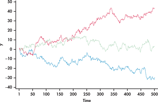
Figure 13.13 shows three simulation runs of our random walk setting for 500 consecutive periods. Notice first that the simulated series look remarkably like stock market charts. In one case (blue line), the random walk series takes a nose dive downward with no indication of returning back. The second case (red line), on the other hand, takes off with the observations steadily increasing. Finally, in the third case (green line), the series wanders around the 0 value. With the first two cases, it would be incorrect to conclude that the processes will continue to trend in the same direction. Moving into the future from , the three random walks can move in any direction, as they did starting from the first period.
659
It should be clear from Example 13.8 that a random walk is anything but random. If we look closely at the random walk model equation, we can gain insights about the random walk process by rearranging terms:
Recognize that represents the change in from one period to the next. In the area of time series, period-to-period changes of a time series are known as first differences. For convenience, define as . This gives us the following relationship:
first differences
Compare this equation with the equation for a random process (page 646). Other than the variable name being here, you should find the equation to be the same. The equation tells us that differences of a random walk follow a random process, with the underlying mean change of the random walk observations being .
Random walk
A random walk is a nonrandom process for which its first differences are random.
If the mean change in the random walk is zero, then the random walk is said to have no drift. With no drift, there is no tendency of the random walk to go in any particular direction, as was seen with the random walk model simulated in Example 13.8. If is not 0, then the random walk is said to have drift. Random walks with will tend to drift upward, while random walks with will tend to drift downward.
EXAMPLE 13.9 Honda Prices
honda1
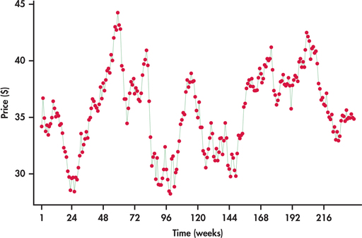
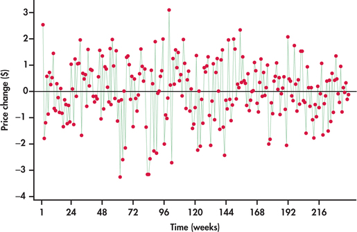
Figure 13.14 plots the weekly closing stock prices of Honda Motor Co. from the beginning of January 2010 through the end of July 2014.5 We can see that the prices are meandering around, much like the green line series of Figure 13.13. The price series is clearly not random. Now consider the first differences of the prices shown in Figure 13.15. The average price change is 0.0029. The price changes are demonstrating random behavior around the average, which implies that the Honda price series is well described by the random walk model.
660
To make a forecast of a future price, we write again the random walk model but shift the subscript one period into the future:
The parameter represents the mean price change. For the Honda series, we find that the sample mean of the price changes is 0.0029. Testing this sample mean against a null hypothesis of , we would find a -value of 0.968; thus, there is not sufficient evidence to reject the null hypothesis. In that light, we proceed with our forecast based on a zero mean price change value. This implies that we are proceeding with a random walk model with no drift. The term represents the future random deviation, which is unknown. If the random deviations have mean 0, our “best” guess for is simply 0. In the end, the forecast equation for predicting Honda’s closing price for time is given by:
In other words, the best forecast of the next period’s price is simply the current period’s price. Using the current observation as the forecast of the next period is known as a naive forecast.
naive forecast
Apply Your Knowledge
Question 13.9
13.9 Honda prices.
Consider the Honda price series of Example 13.9.
- What is the forecast for the closing price one week into the future?
- What is the forecast for the closing price two weeks into the future?
13.9
(a) $34.88. (b) $34.88.
honda1
Question 13.10
13.10 Cleveland financial stress index.
Several of the banks in the Federal Reserve system have developed indices to serve as barometers of the health of the U.S. financial system. For example, the Federal Reserve Bank of Cleveland constructed an index known as the Cleveland Financial Stress Index (CFSI). The CFSI is designed to track distress in the U.S. financial system on a continuous basis. The CFSI tracks stress in six types of markets: credit markets, equity markets, foreign exchange markets, funding markets (interbank markets), real estate markets, and securitization markets. An index reading of zero implies that financial conditions are normal, while a positive reading indicates that the financial system is experiencing some degree of stress. Consider data on daily CFSI readings from January 1, 2014, to August 7, 2014.6
661
- Test the randomness of the CFSI series. What do you conclude?
- Obtain the first differences for the CFSI series and test them for randomness. What do you conclude?
- Would you conclude that the CFSI series behaves as a random walk? Explain.
cfsi
Price changes versus returns
Our discussion of the random walk model centered around the ups and downs of prices. Earlier in Section 13.1, we looked at the ups and downs of Disney prices in terms of percentages. Percentage changes in prices are referred to as returns. The advantage of using returns over price changes is made evident with our next example.
EXAMPLE 13.10 Honda Prices over a Longer Horizon
honda2
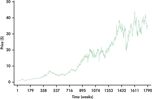
In Example 13.9, we looked at weekly closing prices over an approximate five-year horizon. Consider now the weekly closing prices over a time horizon of more than three decades through the end of July 2014. The price series is shown in Figure 13.16. We can see that the prices started out near 0 and have increased to the range of 30 to 40. Figure 13.17 shows the price changes over this longer time horizon. Though the price changes appear random over time, the salient point with the graph is that the variation of the price changes is increasing substantially with time.
662
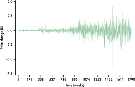
The phenomenon we are witnessing with the increasing variability of price changes is common with economic time series. In particular, many economic time series change as a rate or percentage. Suppose that prices change on average by 1% whether up or down. This would mean that if the price level is $10, the expected price change would be $0.10. But if the price level is at $100, then the expected price change would be $1.00, which is 10 times greater than when the price level was $10.
We can compute returns using the standard formula:
In finance, there can be some ambiguity with the use of the term “return.” It can be defined as the change in price (or value), which, in the preceding formula, is given by the numerator term. But, it is also common practice to have return represent the change in value as a percentage. When return is calculated as a percentage, we could refer to the computed quantity as a “rate of return.” We, however, will go with the standard practice of simply calling the computed values “returns.”
For example, the weekly closing price on July 21, 2014, was $34.99, while the weekly closing price on July 28, 2014, was $34.60. This means the return was
Consider now the following calculation:
The closeness of these values is not accidental. It turns out that the difference of natural logged values is approximately a percent change. We have seen the benefits of the log transformation in many examples. Given these benefits, along with its nice interpretation, it is no wonder we find that so many data analyses in economics and finance are routinely done in logged units.
EXAMPLE 13.11 Honda Returns by Means of Log Transformation
honda2
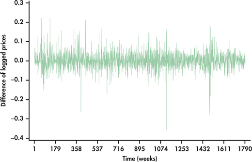
To approximate the percent changes of Honda prices, we first take the log of prices. We then take the differences of the logged values. The differences can be either left in decimal form or multiplied by 100 to be in the form of a percent. Figure 13.18 shows the differences of logged Honda prices left in decimal form. Compare this time plot with the price changes of Figure 13.17. We can clearly see that the returns approximated by the log transformation have much more constant variance. The vertical axis is directly interpretable. For example, we find that weekly returns have dropped as much as 35% and have had increases greater than 20%.
663
The stabilizing effect of the log transformation on the variance of a time series can be quite useful in simplifying modeling efforts. Take a look back at Figure 13.4 (page 648), which shows the time plot of Amazon sales. You should not be surprised that our eventual modeling of this series will involve the log transformation.
Apply Your Knowledge
Question 13.11
13.11 Computing returns.
On August 7, 2014, the S&P 500 closed at 1909.57. On August 8, 2014, the S&P closed at 1931.51.
- Compute the percentage change in the S&P from August 7 to August 8—that is, the daily return as a percentage.
- Approximate the daily return using logs. Compare your answer with part (a).
13.11
(a) 0.011489. (b) 0.011424. The values are quite close.