CHAPTER 14 Review Exercises
For Exercises 14.1 and 14.2, see pages 717–718; for 14.3 and 14.4, see page 720; for 14.5 and 14.6, see page 722; for 14.7, see page 724; for 14.8 and 14.9, see page 726; for 14.10 to 14.13, see pages 728–728; for 14.14 and 14.15, see page 731; for 14.16 to 14.19, see page 739; for 14.20 and 14.21, see page 740; for 14.22 and 14.23, see page 741; for 14.24 and 14.25, see page 742; for 14.26 and 14.27, see page 743; for 14.28 and 14.29, see page 744; and for 14.30 and 14.31, see page 748.
Question 14.32
14.32 A one-way ANOVA example.
A study compared four groups with eight observations per group. An statistic of 2.78 was reported.
- Give the degrees of freedom for this statistic and the entries from Table E that correspond to this distribution.
- Sketch a picture of this distribution with the information from the table included.
- Based on the table information, how would you report the -value?
- Can you reject the null hypothesis that the means are the same at the significance level? Explain your answer.
Question 14.33
14.33 Use the statistic.
A study compared six groups with six observations per group. An statistic of 2.85 was reported.
- Give the degrees of freedom for this statistic and the entries from Table E that correspond to this distribution.
- Sketch a picture of this distribution with the information from the table included.
- Based on the table information, how would you report the -value?
- Can you reject the null hypothesis that the means are the same at the significance level? Explain your answer.
- Can you conclude that all pairs of means are different? Explain your answer.
14.33
(a) . (c) . (d) Reject ; the -value is smaller than . (e) No. A rejection of the null hypothesis only indicates that at least one mean is different, not all.
Question 14.34
14.34 How large does the statistic need to be?
For each of the following situations, state how large the statistic needs to be for rejection of the null hypothesis at the 0.05 level.
- Compare four groups with three observations per group.
- Compare four groups with five observations per group.
- Compare four groups with seven observations per group.
- Summarize what you have learned about distributions from this exercise.
Question 14.35
14.35 Find the statistic.
For each of the following situations, find the statistic and the degrees of freedom. Then draw a sketch of the distribution under the null hypothesis and shade in the portion corresponding to the -value. State how you would report the -value.
- Compare five groups with 13 observations per group, , and .
- Compare three groups with 10 observations per group, , and .
14.35
(a) . (b) .
Question 14.36
14.36 Visualizing the ANOVA model.
For each of the following situations, draw a picture of the ANOVA model similar to Figure 14.6 (page 719). Use numerical values for the . To sketch the Normal curves, you may want to review the 68–95–99.7 rule on page 43.
- and
- and
- and .
Question 14.37
14.37 The ANOVA framework.
For each of the following situations, identify the response variable and the populations to be compared, and give , the , and .
- Last semester, an alcohol awareness program was conducted for three groups of students at an eastern university. Follow-up questionnaires were sent to the participants two months after each presentation. There were 220 responses from students in an elementary statistics course, 145 from a health and safety course, and 76 from a cooperative housing unit. One of the questions was, “Did you discuss the presentation with any of your friends?” The answers were rated on a five-point scale with 1 corresponding to “not at all” and 5 corresponding to “a great deal.”
- A researcher is interested in students’ opinions regarding an additional annual fee to support nonincome-producing varsity sports. Students were asked to rate their acceptance of this fee on a five-point scale. She received 94 responses, of which 31 were from students who attend varsity football or basketball games only, 18 were from students who also attend other varsity competitions, and 45 were from students who did not attend any varsity games.
- A university sandwich shop wants to compare the effects of providing free food with a sandwich order on sales. The experiment will be conducted from 11:00 A.M. to 2:00 P.M. for the next 20 weekdays. On each day, customers will be offered one of the following: a free drink, free chips, a free cookie, or nothing. Each option will be offered five times.
14.37
(a) Response: rating score (1 to 5). The populations are (1) elementary statistics students, (2) health and safety students, and (3) cooperative housing students. . (b) Response: acceptance rating (1 to 5). The populations are (1) students who attend varsity football or basketball games only, (2) students who also attend other varsity competitions, and (3) students who did not attend any varsity games. . (c) Response: sales. The populations are sales on days offering (1) a free drink, (2) free chips, (3) a free cookie, and (4) nothing. .
750
Question 14.38
14.38 Describing the ANOVA model.
For each of the following situations, identify the response variable and the populations to be compared, and give , the , and .
- A developer of a virtual-reality (VR) teaching tool for the deaf wants to compare the effectiveness of different navigation methods. A total of 40 children were available for the experiment, of which equal numbers were randomly assigned to use a joystick, wand, dance mat, or gesture-based pinch gloves. The time (in seconds) to complete a designed VR path is recorded for each child.
- A waiter designed a study to see the effects of his behaviors on the tip amounts that he received. For some customers, he would tell a joke; for others, he would describe two of the food items as being particularly good that night; and for others he would behave normally. Using a table of random numbers, he assigned equal numbers of his next 30 customers to his different behaviors.
- A supermarket wants to compare the effects of providing free samples of cheddar cheese on sales. An experiment will be conducted from 5:00 P.M. to 6:00 P.M. for the next 20 weekdays. On each day, customers will be offered one of the following: a small cube of cheese pierced by a toothpick, a small slice of cheese on a cracker, a cracker with no cheese, or nothing.
Question 14.39
14.39 Provide some details.
Refer to Exercise 14.37. For each situation, give the following:
- Degrees of freedom for group, for error, and for the total.
- Null and alternative hypotheses.
- Numerator and denominator degrees of freedom for the statistic.
14.39
For part a: (a) . (b) not all of the are equal. (c) . For part b: (a) . (b) : not all of the are equal. (c) . For part c: (a) . (b) : not all of the are equal. (c) .
Question 14.40
14.40 Provide some details.
Refer to Exercise 14.38. For each situation, give the following:
- Degrees of freedom for group, for error, and for the total.
- Null and alternative hypotheses.
- Numerator and denominator degrees of freedom for the statistic.
Question 14.41
14.41 How much can you generalize?
Refer to Exercise 14.37. For each situation, discuss the method of obtaining the data and how this would affect the extent to which the results can be generalized.
14.41
Answers will vary. Most situations don’t use random sampling and/or are too specific to be generalizable.
Question 14.42
14.42 How much can you generalize?
Refer to Exercise 14.38. For each situation, discuss the method of obtaining the data and how this would affect the extent to which the results can be generalized.
Question 14.43
14.43 Pooling variances.
An experiment was run to compare four groups. The sample sizes were 30, 32, 150, and 33, and the corresponding estimated standard deviations were 25, 22, 13, and 23.
- Is it reasonable to use the assumption of equal standard deviations when we analyze these data? Give a reason for your answer.
- Give the values of the variances for the four groups.
- Find the pooled variance.
- What is the value of the pooled standard deviation?
- Explain why your answer in part (c) is much closer to the standard deviation for the third group than to any of the other standard deviations.
14.43
(a) Yes, the largest is less than twice the smallest ; . (b) 625, 484, 169, 529. (c) . (d) . (e) The third group has the largest sample size and will influence or weight the pooled standard deviation more.
Question 14.44
14.44 Public transit use and physical activity.
In one study on physical activity, participants used accelerometers and a seven-day travel log to monitor their physical activity.7 Researchers used the data from each participant to quantify the amount of daily walking and to classify each as a non-transit user, or a low-, mid-, or high-frequency transit user. Below is a summary of physical activity (in minutes per day) broken down into walking and non-walking activities.
- Would this be considered an observational study or an experiment? Explain your answer.
- What are the numerator and denominator degrees of freedom for the tests?
- State the null and alternative hypotheses associated with each of the overall -values.
Physical activity Nontransit
Low frequency
Mid frequency
High frequency
Overall
-value
Walking 21.8a 25.8a,b 34.4b,c 36.5c <0.001 Nonwalking 16.0 13.5 11.9 15.2 0.24 - The superscript letters in each row summarize the multiple comparisons results. Write a short paragraph explaining what these results tell you with regard to walking and non-walking physical activity.
751
Question 14.45
14.45 Winery websites.
As part of a study of British Columbia wineries, each of the 193 wineries were classified into one of three categories based on their website features. The Presence stage just had information about the winery. The Portals stage included order placement and online feedback. The Transactions Integration stage included direct payment or payment through a third party online. The researchers then compared the number of market integration features of each winery (for example, in-house touring, a wine shop, a restaurant, in-house wine tasting, gift shop, and so on). Here are the results:8
| Stage | |||
| Presence | 55 | 3.15 | 2.264 |
| Portals | 77 | 4.75 | 2.097 |
| Transactions | 61 | 4.62 | 2.346 |
- Plot the means versus the stage of website. Does there appear to be a difference in the average number of market integration features?
- Is this an observational study or an experiment? Explain your answer.
- Is it reasonable to assume the variances are equal? Justify your reasoning.
- The data are counts (integer values). Also, based on the means and standard deviations, the distributions are skewed (can’t have a negative count). Do you think this lack of Normality poses a problem for ANOVA? Explain your answer.
- The statistic for these data is 9.594. Give the degrees of freedom and -value. What do you conclude?
14.45
(a) The Portals and Transactions stages seem to have higher integration features than the Presence stage. (b) An observational study. They are not imposing a treatment on the winery. (c) Yes, the largest is less than twice the smallest ; . (d) This shouldn’t be a problem because our inference is based on sample means, which will be approximately Normal given the sample sizes. (e) . There are significant differences in the number of market integration features of the wineries among those with different website stages.
Question 14.46
14.46 Time levels of scale.
Recall Exercise 7.62 (page 396). This experiment actually involved three groups. The last group was told the construction project would last 12 months. Here is a summary of the interval lengths (in days) between the earliest and latest completion dates.
timescl
| Group | |||
| 1: 52 weeks | 30 | 84.1 | 55.7 |
| 2: 12 months | 30 | 104.6 | 70.1 |
| 3: 1 year | 30 | 139.6 | 73.1 |
- Is this an observational study or an experiment? Explain your answer.
- Use graphical methods to describe the three populations.
- Examine the conditions necessary for ANOVA. Summarize your findings.
Question 14.47
14.47 Time levels of scale, continued.
Refer to the previous exercise.
timescl
- Run the ANOVA and report the results.
- Use a multiple-comparisons method to compare the three groups. State your conclusions.
- The researchers hypothesized that the more fine-grained the time unit presented to a participant, the smaller the reported interval would be. To test this, they performed a simple linear regression using the group labels 1, 2, and 3 as the predictor variable. They found the slope significantly different from 0 and thus concluded the data supported their hypothesis. Do you think this is an appropriate way to test their hypothesis? Explain your answer.
14.47
(a) not all of the are equal, . There are significant interval differences among the three groups. (b) The Bonferroni procedure shows that group 2 is not significantly different from either group 1 or group 3; however, group 3 is significantly different (larger) than group 1. (c) This is not appropriate. The regression assumes that group 2 (coded as 2) would have twice the effect of group 1 (coded as 1), and group 3 (coded as 3) would have 3 times the effect of group 1, etc. This is likely not true.
Question 14.48
14.48 Additional analysis for the moral strategy example.
CASE 14.1 Refer to Case 14.1 (page 715) for a description of the study and Figure 14.8 (page 724) for the ANOVA results. The researchers hypothesize that the control group would be less likely to continue to buy products because they were not primed with a moral reasoning strategy.
moral
- Because this hypothesis was declared prior to examining the data, can the researchers investigate regardless of the ANOVA test result? Explain your answer.
- Test the alternative hypothesis that the mean of control group is less than the average of the other two groups using . Make sure to specify the contrast coefficients, the contrast estimate, the contrast standard error, degrees of freedom, and -value.
Question 14.49
14.49 Additional ANOVA for the moral strategy example.
Refer to Case 14.1 (page 715) for a description of the study. In addition to rating the likelihood to continue to purchase products, each participant was also asked to judge the CEO’s degree of immorality. This was done by answering a couple questions on a 0–7 scale where the high the score, the stronger the immorality.
moral1
- Use numerical and graphical methods to describe the three populations.
- Examine the conditions necessary for ANOVA. Summarize your findings.
- Run the ANOVA and report the results.
14.49
(a)
| Immorality | |||
|---|---|---|---|
| Level of Grp |
Mean | Std Dev | |
| C | 41 | 6.4512 | 0.5788 |
| D | 43 | 6.2209 | 0.8040 |
| R | 37 | 5.6892 | 1.2767 |
(b) There is no reason to believe the cases are not independent. Constant variance is violated: the largest is more than twice the smallest , . The sample sizes are large enough that the sample means should be approximately Normally distributed. ANOVA should not be used because the standard deviations are too different to be assumed equal. (c) not all of the are equal, . There are significant immorality judgment differences among the three groups.
Question 14.50
14.50 Additional ANOVA for the moral strategy example, continued.
Refer to the previous exercise.
moral1
- Use a multiple-comparisons method to compare the three groups. State your conclusions.
- Refer to the results in Exercise 14.48 and part (a). The researchers hypothesized that moral decoupling would allow a participant to view the behavior as immoral yet still be likely to to purchase products. Does this group appear to be the only one with this behavior? Generate a numerical or graphical summary that helps explain your answer to this question.
752
Question 14.51
14.51 Organic foods and morals?
Organic foods are often marketed using moral terms such as “honesty” and “purity.” Is this just a marketing strategy, or is there a conceptual link between organic food and morality? In one experiment, 62 undergraduates were randomly assigned to one of three food conditions (organic, comfort, and control).9 First, each participant was given a packet of four food types from the assigned condition and told to rate the desirability of each food on a 7-point scale. Then, each was presented with a list of six moral transgressions and asked to rate each on a 7-point scale ranging from 1 = not at all morally wrong to 7 = very morally wrong. The average of these six scores was used as the response.
organic
- Make a table giving the sample size, mean, and standard deviation for each group. Is it reasonable to pool the variances?
- Generate a histogram for each of the groups. Can we feel confident that the sample means are approximately Normal? Explain your answer.
14.51
(a)
| Score | |||
|---|---|---|---|
| Level of Food |
Mean | Std Dev | |
| Comfort | 22 | 4.8873 | 0.5729 |
| Control | 20 | 5.0825 | 0.6217 |
| Organic | 35 | 5.5835 | 0.5936 |
Yes, the largest is less than twice the smallest ; . (b) While the distributions aren’t Normal, there are no outliers or extreme departures from Normality that would invalidate the results. We can likely proceed with the ANOVA.
Question 14.52
14.52 Organic foods and morals, continued.
Refer to the previous exercise.
organic
- Analyze the scores using analysis of variance. Report the test statistic, degrees of freedom, and -value.
- Assess the assumptions necessary for inference by examining the residuals. Summarize your findings.
- Compare the groups using the least-significant differences method.
- A higher score is associated with a harsher moral judgment. Using the results from parts (a) and (c), write a short summary of your conclusions.
Question 14.53
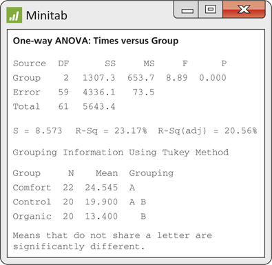
14.53 Organic foods and friendly behavior?
Refer to Exercise 14.51 for the design of the experiment. After rating the moral transgressions, the participants were told “that another professor from another department is also conducting research and really needs volunteers.” They were told that they would not receive compensation or course credit for their help and then were asked to write down the number of minutes (out of 30) that they would be willing to volunteer. This sort of question is often used to measure a person’s prosocial behavior.
organic
- Figure 14.19 contains the Minitab output for the analysis of this response variable. Write a one-paragraph summary of your conclusions.
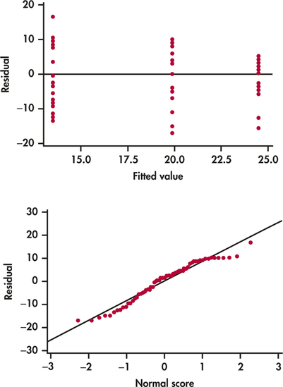
- Figure 14.20 contains a residual plot and a Normal quantile plot of the residuals. Are there any concerns regarding the assumptions necessary for inference? Explain your answer.
14.53
(a) not all of the are equal, . There are significant differences in the number of minutes that the three groups are willing to volunteer. According to the Tukey multiple comparison, the Comfort group is willing to donate significantly more minutes than the Organic group. In other words, the Comfort group shows more prosocial behavior than the Organic group. The Control group is in the middle, not significantly different from either the Comfort or Organic group in the number of minutes they are willing to donate. (b) The residual plot shows a slight decrease in variability, suggesting a possible violation of constant variance. The Normal quantile plot looks fine and shows a roughly Normal distribution.
753
Question 14.54
14.54 Restaurant ambiance and consumer behavior.
There have been numerous studies investigating the effects of restaurant ambiance on consumer behavior. One study investigated the effects of musical genre on consumer spending.10 At a single high-end restaurant in England over a three-week period, there were a total of 141 participants; 49 of them were subjected to background pop music while dining, 44 to background classical music, and 48 to no background music. For each participant, the total food bill (in British pounds), adjusted for time spent dining, was recorded. The following table summarizes the means and standard deviations.
| Background music |
|||
| Pop | 21.912 | 49 | 2.627 |
| Classical | 24.130 | 44 | 2.243 |
| None | 21.697 | 48 | 3.332 |
| Total | 22.531 | 141 | 2.969 |
- Plot the means versus the type of background music. Does there appear to be a difference in spending?
- Is it reasonable to assume that the variances are equal? Explain.
- The statistic is 10.62. Give the degrees of freedom and either an approximate (from a table) or an exact (from software) -value. What do you conclude?
- Refer back to part (a). Without doing any formal analysis, describe the pattern in the means that is likely responsible for your conclusion in part (c).
- To what extent do you think the results of this study can be generalized to other settings? Give reasons for your answer.
Question 14.55
14.55 Shopping and bargaining in Mexico.
Price haggling and other bargaining behaviors among consumers have been observed for a long time. However, research addressing these behaviors, especially in a real-life setting, remains relatively sparse. A group of researchers recently performed a small study to determine whether gender or nationality of the bargainer has an effect on the final price obtained.11 The study took place in Mexico because of the prevalence of price haggling in informal markets. Salespersons working at various informal shops were approached by one of three bargainers looking for a specific product. After an initial price was stated by the vendor, bargaining took place. The response was the difference between the initial and the final price of the product. The bargainers were a Spanish-speaking Hispanic male, a Spanish-speaking Hispanic female, and an Anglo non-Spanish-speaking male. The following table summarizes the results.
| Bargainer | ||
| Hispanic male | 40 | 1.055 |
| Hispanic female | 40 | 2.310 |
| Anglo male | 40 | 1.050 |
- To compare the mean reductions in price, what are the degrees of freedom for the ANOVA statistic?
- The reported test statistic is . Give an approximate (from a table) or exact (from software) -value. What do you conclude?
- To what extent do you think the results of this study can be generalized? Give reasons for your answer.
14.55
(a) . (b) . There are significant average reduction differences among the different groups of bargainers. (c) Because the bargainer was the same person each time, there is no way to differentiate if the average reduction was due to race/gender or due to individual ability to bargain. Hence, the results would certainly not be generalizable.
Question 14.56
14.56 Internet banking.
A study in Finland looked at consumer perceptions of Internet banking (IB).12 Data were collected via personal, structured interviews as part of a nationwide consumer study. The sample included 300 active users of IB, between 15 and 74 years old. Based on the survey, users were broken down into three groups based on their familiarity with the Internet. For this exercise, we consider the consumer’s perception of status or image in the eyes of other consumers. Standardized scores were used for analysis.
| Familiarity | Mean | |
| Low | 0.21 | 77 |
| Medium | −0.14 | 133 |
| High | 0.03 | 90 |
- To compare the mean scores across familiarity levels, what are the degrees of freedom for the ANOVA statistic?
- The . If , what is the statistic?
- Give an approximate (from a table) or exact (from software) -value. What do you conclude?
Question 14.57
14.57 The multiple-play strategy.
Multiple play is a bundling strategy in which multiple services are provided over a single network. A common triple-play service these days is Internet, television, and telephone. The market for this service has become a key battleground among telecommunication, cable, and broadband service providers. A recent study compared the pricing (in dollars) among triple-play providers using DSL, cable, or fiber platforms.13 The following table summarizes the results from 47 providers.
754
| Group | |||
| DSL | 19 | 104.49 | 26.09 |
| Cable | 20 | 119.98 | 40.39 |
| Fiber | 8 | 83.87 | 31.78 |
- Plot the means versus the platform type. Does there appear to be a difference in pricing?
- Is it reasonable to assume that the variances are equal? Explain.
- The statistic is 3.39. Give the degrees of freedom and either an approximate (from a table) or an exact (from software) -value. What do you conclude?
14.57
(a) The pricing among triple-play providers does seem different. Cable has the highest prices followed by DSL. Fiber has the cheapest prices for tripleplay. (b) Yes, the largest is less than twice the smallest ; . (c) . There are significant differences in triple-play pricing among the difference provider platforms.
Question 14.58
14.58 A contrast.
Refer to the previous exercise. Use a contrast to compare the fiber platform with the average of the other two. The hypothesis prior to collecting the data is that the fiber platform price would be smaller. Summarize your conclusion.
Question 14.59
14.59 Financial incentives for weight loss.
The use of financial incentives has shown promise in promoting weight loss and healthy behaviors. In one study, 104 employees of the Children’s Hospital of Philadelphia, with BMIs of 30 to 40 kilograms per square meter , were each randomly assigned to one of three weight-loss programs.14 Participants in the control program were provided a link to weight-control information. Participants in the individual-incentive program received this link but were also told that $100 would be given to them each time they met or exceeded their target monthly weight loss. Finally, participants in the group-incentive program received similar information and financial incentives as the individual-incentive program but were also told that they were placed in secret groups of five and at the end of each four-week period, those in their group who met their goals throughout the period would equally split an additional $500. The study ran for 24 weeks and the total change in weight (in pounds) was recorded.
loss
- Make a table giving the sample size, mean, and standard deviation for each group.
- Is it reasonable to pool the variances? Explain your answer.
- Generate a histogram for each of the programs. Can we feel confident that the sample means are approximately Normal? Defend your answer.
14.59
(a)
| Loss | |||
|---|---|---|---|
| Level of Group | Mean | Std Dev | |
| Ctrl | 35 | −1.0086 | 11.5007 |
| Grp | 34 | −10.7853 | 11.1392 |
| Indiv | 35 | −3.7086 | 9.0784 |
(b) Yes, the largest is less than twice the smallest ; . (c) All three distributions are roughly Normal.
Question 14.60
14.60 Financial incentives for weight loss, continued.
Refer to the previous exercise.
loss
- Analyze the change in weight using analysis of variance. Report the test statistic, degrees of freedom, -value, and your conclusions.
- Even though you assessed the model assumptions in the previous exercise, let’s check the assumptions again by examining the residuals. Summarize your findings.
- Compare the groups using the least-significant difference method.
- Using the results from parts (a), (b), and (c), write a short summary of your conclusions.
Question 14.61
14.61 Changing the response variable.
Refer to the previous two exercises, where we compared three weight-loss programs using change in weight measured in pounds. Suppose that you decide to instead make the comparison using change in weight measured in kilograms.
loss
- Convert the weight loss from pounds to kilograms by dividing each response by 2.2.
- Analyze these new weight changes using analysis of variance. Compare the test statistic, degrees of freedom, and -value you obtain here with those reported in part (a) of the previous exercise. Summarize what you find.
14.61
(a) All weight loss values are divided by 2.2. (b) and . The results are identical with the transformed data regarding the test statistic, DF, and -value. Transforming the response variable by a fixed amount has no effect on the ANOVA results.
Question 14.62
14.62 Does sleep deprivation affect your work?
Sleep deprivation experienced by physicians during residency training and the possible negative consequences are of concern to many in the health care community. One study of 33 resident anesthesiologists compared their changes from baseline in reaction times on four tasks.15 Under baseline conditions, the physicians reported getting an average of 7.04 hours of sleep. While on duty, however, the average was 1.66 hours. For each of the tasks, the researchers reported a statistically significant increase in the reaction time when the residents were working in a state of sleep deprivation.
- If each task is analyzed separately as the researchers did in their report, what is the appropriate statistical method to use? Explain your answer.
- Is it appropriate to use a one-way ANOVA with to analyze these data? Explain why or why not.
Question 14.63
14.63 Promotions and the expected price of a product.
If a supermarket product is frequently offered at a reduced price, do customers expect the price of the product to be lower in the future? This question was examined by researchers in a study conducted on students enrolled in an introductory management course at a large midwestern university. For 10 weeks, 160 subjects read weekly ads for the same product. Students were randomly assigned to read one, three, five, or seven ads featuring price promotions during the 10-week period. They were then asked to estimate what the product’s price would be the following week.16 Table 14.1 gives the data.
ppromo
755
- Make a Normal quantile plot for the data in each of the four treatment groups. Summarize the information in the plots and draw a conclusion regarding the Normality of these data.
- Summarize the data with a table containing the sample size, mean, and standard deviation for each group.
- Is the assumption of equal standard deviations reasonable here? Explain why or why not.
- Carry out a one-way ANOVA. Give the hypotheses, the test statistic with its degrees of freedom, and the -value. Summarize your conclusion.
14.63
(a) All four Normal quantile plots show roughly Normal distributions with only minor departures from Normality.
(b)
| Price | |||
|---|---|---|---|
| Level of Promotions | Mean | Std Dev | |
| 1 | 40 | 4.2240 | 0.2734 |
| 3 | 40 | 4.0628 | 0.1742 |
| 5 | 40 | 3.7590 | 0.2526 |
| 7 | 40 | 3.5488 | 0.2750 |
(c) Yes, the largest is less than twice the smallest ; . (d) : not all of the are equal, . There are significant price estimate differences among the four groups, which read different numbers of promotions.
Question 14.64
14.64 Compare the means.
Refer to the previous exercise. Use the Bonferroni or another multiple-comparisons procedure to compare the group means. Summarize the results and support your conclusions with a graph of the means.
ppromo
Question 14.65
14.65 Considering a transformation.
CASE 14.1 In Example 14.8 (pages 723–724), we compared the likelihood to purchase among three groups. We performed ANOVA, even though the data were non-Normal with possible nonconstant variance, because of the robustness of the procedure. For this exercise, let’s consider a transformation.
moral
- We have data that must be between 0 and 100. This kind of constraint can result in skewed distributions and unequal variances in a similar fashion to the binomial distribution as moves away from 0.5 toward 0 or 1. For data like these, there is a special transformation, the arcsine square root transformation, that often is helpful. Construct this new response variable
- Construct histograms of this response variable for each population. Compare the distributions of the transformed variable with those in Figure 14.3 (page 716). Does the spread appear more similar? Do the data also look more Normal?
- Perform ANOVA on the transformed variable. Do the results vary much from those in Figure 14.8?
14.65
(b) The distributions of the transformed data are much more Normal than the original likelihood histograms. The spreads are all very similar now between 0.2 and 0.25. (c) . There are significant differences among groups for the transformed data. The results of this ANOVA are quite similar to the results of the ANOVA on the untransformed data.
Question 14.66
14.66 Comparing confidence intervals.
CASE 14.1 Refer to the previous exercise.
moral
- Construct simultaneous confidence interval for the average difference in purchase likelihood between the moral decoupling group and the control group.
- Construct the simultaneous confidence interval for the average difference in transformed purchase likelihood between the moral decoupling group and the control group.Table 14.23: TABLE 14.1 Price promotion data
Number of
promotionsExpected price (dollars) 1 3.78 3.82 4.18 4.46 4.31 4.56 4.36 4.54 3.89 4.13 3.97 4.38 3.98 3.91 4.34 4.24 4.22 4.32 3.96 4.73 3.62 4.27 4.79 4.58 4.46 4.18 4.40 4.36 4.37 4.23 4.06 3.86 4.26 4.33 4.10 3.94 3.97 4.60 4.50 4.00 3 4.12 3.91 3.96 4.22 3.88 4.14 4.17 4.07 4.16 4.12 3.84 4.01 4.42 4.01 3.84 3.95 4.26 3.95 4.30 4.33 4.17 3.97 4.32 3.87 3.91 4.21 3.86 4.14 3.93 4.08 4.07 4.08 3.95 3.92 4.36 4.05 3.96 4.29 3.60 4.11 5 3.32 3.86 4.15 3.65 3.71 3.78 3.93 3.73 3.71 4.10 3.69 3.83 3.58 4.08 3.99 3.72 4.41 4.12 3.73 3.56 3.25 3.76 3.56 3.48 3.47 3.58 3.76 3.57 3.87 3.92 3.39 3.54 3.86 3.77 4.37 3.77 3.81 3.71 3.58 3.69 7 3.45 3.64 3.37 3.27 3.58 4.01 3.67 3.74 3.50 3.60 3.97 3.57 3.50 3.81 3.55 3.08 3.78 3.86 3.29 3.77 3.25 3.07 3.21 3.55 3.23 2.97 3.86 3.14 3.43 3.84 3.65 3.45 3.73 3.12 3.82 3.70 3.46 3.73 3.79 3.94 756
- We can’t directly compare the two intervals because they are on a different scale. Backtransform the upper and lower endpoints of your confidence interval in part (b). This is done by taking the sine of each endpoint, squaring them, and then multiplying by 100.
- Now compare the confidence intervals in parts (a) and (c). Write a summary paragraph explaining which interval you prefer.
Question 14.67
14.67 Word-of-mouth communications.
Consumers often seek opinions on products from other consumers. These word-of-mouth communications are considered valuable because they are thought to be less biased toward the product and more likely to contain negative information. What makes certain opinions with negative information more credible than others? A group of researchers think it may have to do with the use of dispreferred markers. Dispreferred markers indicate that the communicator has just said, or is about to say, something unpleasant or negative. To investigate this they recruited 257 subjects and randomly assigned them to three groups: positive-only review, balanced review, and balanced review with a dispreferred marker. Each subject read about two friends discussing one of their cars. The positive-only group heard that it has been owned for three years, rides well, and gets good gas mileage. The other two groups also hear that the radio and air conditioner cannot run at the same time.17 One of the variables measured is the credibility of the friend describing her car. Here is part of the ANOVA table for these data:
| Source | Degrees of freedom |
Sum of squares |
Mean square |
|
| Groups | 183.59 | |||
| Error | 2643.53 | |||
| Total | 256 |
- Fill in the missing entries in the ANOVA table.
- State and for this experiment.
- What is the distribution of the statistic under the assumption that is true? Using Table E, give an approximate -value for the ANOVA test. Write a brief conclusion.
- What is , the estimate of the within-group variance? What is the pooled standard error ?
14.67
(a) . (b) : not all of the are equal. (c) . There are significant differences among the groups. (d) .
Question 14.68
14.68 Word-of-mouth communications, continued.
Another variable measured in the experiment described in the previous exercise was the likability of the friend describing her car. Higher values of this score indicate a better opinion. Here is part of the ANOVA table for these data:
| Source | Degrees of freedom |
Sum of squares |
Mean square |
|
| Groups | 9.20 | |||
| Error | 0.93 | |||
| Total | 256 |
- Fill in the missing entries in the ANOVA table.
- State and for this experiment.
- What is the distribution of the statistic under the assumption that is true? Using Table E, give an approximate -value for the ANOVA test. What do you conclude?
- What is , the estimate of the within-group variance? What is ?
Question 14.69
14.69 Writing contrasts.
Return to the eye study described in Example 14.13 (pages 729–731). Let , and represent the mean scores for blue, brown, gaze down, and green eyes.
- Because a majority of the population is Hispanic (eye color predominantly brown), we want to compare the average score of the brown eyes with the average of the other two eye colors. Write a contrast that expresses this comparison.
- Write a contrast to compare the average score when the model is looking at you versus the score when looking down.
14.69
(a) . (b) .
Question 14.70
14.70 Writing contrasts.
You’ve been asked to help some administrators analyze survey data on textbook expenditures collected at a large public university. Let , and represent the population mean expenditures on textbooks for the freshmen, sophomores, juniors, and seniors, respectively.
- Because juniors and seniors take higher-level courses, which might use more expensive textbooks, the administrators want to compare the average of the freshmen and sophomores with the average of the juniors and seniors. Write a contrast that expresses this comparison.
- Write a contrast for comparing the freshmen with the sophomores.
- Write a contrast for comparing the juniors with the seniors.
Question 14.71
14.71 Analyzing contrasts.
Return to the eyes study in Example 14.13 (pages 729–731). Answer the following questions for the two contrasts that you defined in Exercise 14.69.
- For each contrast give and an appropriate . In choosing the alternatives, you should use information given in the description of the problem, but you may not consider any impressions obtained by inspection of the sample means.
757
- Find the values of the corresponding sample contrasts and .
- Using the value , calculate the standard errors and for the sample contrasts.
- Give the test statistics and approximate -values for the two significance tests. What do you conclude?
- Compute 95% confidence intervals for the two contrasts.
14.71
For part a: (a) . (Arguments could be made for a one-sided alternative as well.) (b) . (c) . (d) . There is not enough evidence that the average score of the brown eyes is different than the average score of the other two eye colors. (e) . For part b: (a) . (Arguments could be made for a one-sided alternative as well.) (b) . (c) . (d) . There is not enough evidence that the average score when the model is looking at you is different than the average score when the model is looking down. (e) .
Question 14.72
14.72 The effect of increased sample size.
Set the standard deviation for the One-Way ANOVA applet at a middle value and drag the black dots so that the means are roughly 5.00, 4.50, and 5.25.

- What are the statistic, its degrees of freedom, and the -value?
- Slide the sample size bar to the right so . Also drag the black dots back to the values of 5.00, 4.50, and 5.25. What are the statistic, its degrees of freedom and the -value?
- Explain why the statistic and -value change in this way as increases.
Question 14.73
14.73 Power for the weight-loss study.
You are planning another study of financial incentives for weight-loss study similar to that described in Exercise 14.59 (page 754). The standard deviations given in that exercise range from 9.08 to 11.50. To perform power calculations, assume that the standard deviation is . You have three groups, each with subjects, and you would like to reject the ANOVA when the alternative , and is true. Use software to make a table of powers against this alternative (similar to the table in Example 14.28, page 748) for the following numbers in each group: , and 75. What sample size would you choose for your study?
14.73
Answers will vary; or 75 would be good choices.
| DFG | DFE | F* | Power | |
|---|---|---|---|---|
| 35 | 2 | 102 | 3.09 | 0.609 |
| 45 | 2 | 132 | 3.06 | 0.729 |
| 55 | 2 | 162 | 3.05 | 0.818 |
| 65 | 2 | 192 | 3.04 | 0.881 |
| 75 | 2 | 222 | 3.04 | 0.924 |
Question 14.74
14.74 Same power?
Repeat the previous exercise for the alternative , and . Why are the results the same?
Question 14.75
14.75 Planning another organic foods study.
Suppose that you are planning a new organic foods study using the same moral outcome variable as described in Exercise 14.51 (page 752). Your study will randomly choose shoppers from a large local grocery store.
- Explain how you would select the shoppers to participate in your study.
- Use the data from Exercise 14.51 (page 752) to perform power calculations to determine sample sizes for your study.
- Write a report that could be understood by someone with limited background in statistics and that describes your proposed study and why you think it is likely that you will obtain interesting results.
14.75
(a) Answers will vary.
| DFG | DFE | F* | Power | |
|---|---|---|---|---|
| 10 | 2 | 27 | 3.35 | 0.621 |
| 15 | 2 | 42 | 3.22 | 0.821 |
| 20 | 2 | 57 | 3.16 | 0.924 |
| 25 | 2 | 72 | 3.12 | 0.97 |
| 30 | 2 | 87 | 3.10 | 0.989 |
(b) For , the power is already 0.924. (c) Answers will vary.
Question 14.76
14.76 Planning another restaurant ambiance study.
Exercise 14.54 (page 753) gave data for a study that examined the effect of background music on total food spending at a high-end restaurant. You are planning a similar study but intend to look at total food spending at a more casual restaurant. Use the results of the study described in Exercise 14.54 to plan your study. Write a short one- to two-paragraph proposal detailing your experiment.
Question 14.77
14.77 The effect of an outlier.
Refer to the weight-loss study described in Exercise 14.59 (page 754).
loss
- Suppose that when entering the data into the computer, you accidentlly entered the first observation as 53 pounds rather than 5.3 pounds. Run the ANOVA with this incorrect observation, and record the statistic, the estimate of the within-group variance , and the estimated treatment means.
- Alternatively, suppose that when entering the data into the computer, you accidentally entered Observation #101 as 79.4 pounds rather than 19.4 pounds. Run the ANOVA with this incorrect observation, and record the same information requested in part (a).
- Compare the results of each of these two cases with the results obtained with the correct data set. What happens to the within-group variance ? Do the estimated treatment means move closer or further apart? What effect do these changes have on the test?
- What do these two cases illustrate about the effects of an outlier in an ANOVA? Write a one-paragraph summary.
- Explain why a table of means and standard deviations for each of the three treatments would help you to detect an incorrect observation.
14.77
(a) The results are nearly identical as before: .
| Loss | |||
|---|---|---|---|
| Level of Group |
Mean | Std Dev | |
| Ctrl | 35 | 0.3543 | 14.6621 |
| Grp | 34 | −10.7853 | 11.1392 |
| Indiv | 35 | −3.7086 | 9.0784 |
(b) The results are not as significant: .
| Loss | |||
|---|---|---|---|
| Level of Group |
Mean | Std Dev | |
| Ctrl | 35 | −1.0086 | 11.5007 |
| Grp | 34 | −9.0206 | 18.4317 |
| Indiv | 35 | −3.7086 | 9.0784 |
(c) With the first outlier, the means got farther apart, suggesting more significance, but the estimated variance went from 112.81 to 140.65, suggesting a worse fit, which resulted in a very similar and -value. With the second outlier, the means got closer together, suggesting less significance, and the estimated variance went from 112.81 to 183.27, also suggesting a much worse fit, which resulted in a -value much less significant than originally and almost not significant. In both cases, the estimate variance got much worse, so generally outliers should make it harder to so see significance. But as shown in the first example, if the outlier pulls the means farther apart, this may not be true. (d) We can see the incorrect observation because the standard deviation for the group with the outlier becomes much larger than the standard deviations for the other groups.
Question 14.78
14.78 Changing units and ANOVA.
Refer to Exercise 14.61 (page 754). Suggest a general conclusion about what happens to the test statistic, degrees of freedom, -value, and conclusion when you perform ANOVA on data after changing the units through a linear transformation , where and are chosen constants. In Exercise 14.61, the constants were and .
Question 14.79
14.79 Regression or ANOVA?
Refer to the price promotion study that we examined in Exercise 14.63 (pages 754–755). The explanatory variable in this study is the number of price promotions in a 10-week period, with possible values of 1, 3, 5, and 7. ANOVA treats the explanatory variable as categorical—it just labels the groups to be compared. In this study, the explanatory variable is, in fact, quantitative, so we could use simple linear regression rather than one-way ANOVA if there is a linear pattern.
ppromo
758
- Make a scatterplot of the responses against the explanatory variable. Is the pattern roughly linear?
- In ANOVA, the test null hypothesis states that groups have no effect on the mean response. What test in regression tests the null hypothesis that the explanatory variable has no linear relationship with the response?
- Carry out the regression. Compare your results with those from the ANOVA in Exercise 14.63. Are there any reasons—perhaps from part (a)—to prefer one or the other analysis?
14.79
(a) The pattern is roughly linear. (b) Testing the slope equal to zero is the test of no linear relationship. (c) . There is a significant linear relationship between price and the number of promotions. Because the relationship is linear as shown in part (a), the regression is preferable because it not only says that the number of promotions affects price, but also describes the relationship as a linear one, in which we can quantify the relationship by interpreting the slope. In this problem, for each additional promotion read, the expected price goes down by 0.11648.
Question 14.80
14.80 Pooling variances, continued.
Refer to Exercise 14.43 (page 750). Based on our rule of thumb (page 720), we consider it reasonable to use the assumption of equal standard deviations in our analysis. However, when sample sizes vary substantially, we need to use caution. As demonstrated in Exercise 14.43, the pooled standard deviation is closer to the standard deviation of the third group than any of the other three standard deviations. Assuming these sample standard deviations are close to the population standard deviations, explain the impact of using the pooled standard deviation on the coverage of the simultaneous confidence intervals between means. In particular, would you expect the coverage of the interval for the difference between the first and second group to be larger or smaller than ? Explain your answer.