15.1 The Two-Way ANOVA Model
15-2
We begin with a discussion of the advantages of the two-way ANOVA design and illustrate these with some examples. Then we discuss the model and the conditions that justify two-way ANOVA.
Advantages of two-way ANOVA
In one-way ANOVA, we classify populations according to one categorical variable, or factor. In the two-way ANOVA model, there are two factors, each with several levels. When we are interested in the effects of two factors, a two-way design offers great advantages over two single-factor studies. We use several examples to illustrate these advantages.
factor
EXAMPLE 15.1 Experimental Design 1: Best Magazine Layout and Cover
In Example 14.1 (page 712), a magazine publisher wants to compare three different magazine layouts. To do this, she plans to randomly assign the three design layouts equally among 60 supermarkets. The number of magazines sold during a one-week period is the outcome variable.
Now suppose a second experiment is planned for the following week to compare four different covers for the magazine. A similar experimental design will be used, with the four covers randomly assigned equally among the same 60 supermarkets.
Here is the design of the first experiment with the sample sizes:
| Layout | |
| 1 | 20 |
| 2 | 20 |
| 3 | 20 |
| Total | 60 |
And here is the second experiment:
| Cover | |
| 1 | 15 |
| 2 | 15 |
| 3 | 15 |
| 4 | 15 |
| Total | 60 |
In the first experiment, 20 stores were assigned to each level of the factor for a total of 60 stores. In the second experiment 15 stores were assigned to each level of the factor for a total of 60 stores. Each experiment lasts one week, so the total amount of time for the two experiments is two weeks.
Each experiment will be analyzed using one-way ANOVA. The factor in the first experiment is magazine layout with three levels, and the factor in the second experiment is magazine cover with four levels. Let’s now consider combining the two experiments into one.
15-3
EXAMPLE 15.2 Experimental Design 2: Best Magazine Layout and Cover
Suppose we use a two-way approach for the magazine design problem. There are two factors, layout and cover. Because layout has three levels and cover has four levels, this is a design. This gives a total of 12 possible combinations of layout and cover. With a total of 60 stores, we could assign each combination of layout and cover to five stores. The number of magazines sold during a one-week period is the outcome variable.
Here is a picture of the two-way design with the sample sizes:
| Cover | |||||
| Layout | 1 | 2 | 3 | 4 | Total |
| 1 | 5 | 5 | 5 | 5 | 20 |
| 2 | 5 | 5 | 5 | 5 | 20 |
| 3 | 5 | 5 | 5 | 5 | 20 |
| Total | 15 | 15 | 15 | 15 | 60 |
Each combination of the factors in a two-way design corresponds to a cell. The ANOVA for the magazine experiment has 12 cells, each corresponding to a particular combination of layout and cover.
cell
With the two-way design for layout and cover, notice that we have 20 stores assigned to each level, the same as we had for the one-way experiment for layout alone. Similarly, there are 15 stores assigned to each level of cover. Thus, the two-way design gives us the same amount of information for estimating the sales for each level of each factor as we had with the two one-way designs. The difference is that we can collect all the information in only one experiment. This experiment lasts one week (instead of two weeks) and involves a single observation from each of the 60 stores. By combining the two factors into one experiment, we have increased our efficiency by reducing the amount of data to be collected by half.
EXAMPLE 15.3 Bundling to Introduce a New Product
Bundling is a marketing strategy that involves the sale of two or more separate products in one package. It is frequently used to introduce a new product or brand. For example, a new hair gel might be bundled with a popular shampoo, or a new cell phone might be bundled with a new wireless service contract. While much research has been done in terms of evaluating the quality of a bundle, relatively little has been done on the effects of bundling. Do the characteristics of the partnered product affect a consumer’s opinion of the new product? One characteristic of interest would be the partnered product’s functional relatedness, or complementarity.3 If the partnered product is used in conjunction with the new product, does that enhance the consumer’s perception of the new product?
To design a study to answer this question, we first need to determine an appropriate target group. This will depend on the new product under consideration. Suppose we’re interested in introducing a new surround sound receiver and, therefore, decide to focus on college-age consumers of electronics. For our partnered products, we decide on a six-piece speaker system as the complementary product and a digital camera as the noncomplementary product. Because consumers have been shown to respond differently to products based on the product’s brand image, our design should also take that into account. Let’s consider a two-way ANOVA for this study.
15-4
EXAMPLE 15.4 Two-Way Design for the Bundling Study
The factors for this two-way ANOVA are the partnered product’s complementarity and brand image, each with two levels. There are cells in this study. If 200 consumers were recruited, we would then randomly assign 50 to each cell. The outcome variable will be a measure of the new product’s image based on several 7-point scale questions.
Here is a table that summarizes the design:
| Complementarity | |||
| Brand image | Low | High | Total |
| Low | 50 | 50 | 100 |
| High | 50 | 50 | 100 |
| Total | 100 | 100 | 200 |
This example illustrates a second reason for using two-way designs. Although we’re primarily interested in the effect of the partnered product’s complementarity, we included the partnered product’s brand image because we thought there might be an effect. Consider an alternative, one-way design where we assign 200 consumers to the two levels of complementarity and ignore brand image. With this design, we have the same number of consumers at each of the complementarity levels; thus, in this way, it is similar to our two-way design. However, suppose that there is, in fact, an effect of brand image. In this case, the one-way ANOVA would assign this variation to the RESIDUAL (within groups) part of the model. In the two-way ANOVA, brand image is included as a factor, and therefore this variation is included in the FIT part of the model. Whenever we can move variation from RESIDUAL to FIT, we reduce the of our model and increase the power of our tests.
Reminder

p. 489
EXAMPLE 15.5 Disorganized Shelf Display and Product Availability
Despite a retailer’s best efforts, products displayed on shelves can become disorganized and scarce. Does this affect the purchase likelihood of a product? Researchers consider the impact of shelf display (organized or disorganized) and product quantity (low, medium, high) on the purchase likelihood of a snack food product.4
Suppose we wanted to compare an organized and disorganized shelf display across three different product quantity levels. Instead of three separate one-way ANOVAs (or two-sample tests), one for each quantity level, we make product quantity a factor in our design.
EXAMPLE 15.6 Two-Way Design for the Shelf Display Study
We use a design for our shelf display study. The two factors are shelf display organization and product quantity. For product quantity, we compare the levels low (or scarce), medium, and high. The study that this example is based on used a convenience sample of undergraduate students taking a marketing class. Although aware of the potential hazards with this type of sampling, we obtain 72 student volunteers from our university. Each student is randomly shown one of six pictures of the shelf display. We measure purchase intent through a series of questions that are scored on a 1 to 7 scale.
15-5
Here is a table that summarizes the design with the sample sizes:
| Shelf display | |||
| Product quantity | Organized | Disorganized | Total |
| Low | 12 | 12 | 24 |
| Medium | 12 | 12 | 24 |
| High | 12 | 12 | 24 |
| Total | 36 | 36 | 72 |
This example illustrates a third reason for using two-way designs. The difference between the two shelf displays may depend on the product quantity. We call this an interaction when it occurs. In contrast, the average values for the shelf display effect and the product quantity effect are represented as main effects. The two-way model represents FIT as the sum of a main effect for each of the two factors and an interaction. One-way designs that vary a single factor and hold other factors fixed cannot discover interactions. We discuss interactions more fully later in this section.
interaction
main effects
These examples illustrate several reasons why two-way designs are preferable to one-way designs.
Advantages of Two-Way ANOVA
- It is more efficient to study two factors simultaneously rather than separately.
- We can reduce the residual variation in a model by including a second factor thought to influence the response.
- We can investigate interactions between factors.
These considerations also apply to study designs with more than two factors. We are content to explore only the two-way case. The choice of the design for data production (sample or experiment) is fundamental to any statistical study. Factors and levels must be carefully selected by an individual or team who understands both the statistical models and the issues that the study will address.
The two-way ANOVA model
When discussing two-way models in general, we use the labels A and B for the two factors. For particular examples and when using statistical software, it is better to use names for these categorical variables that suggest their meaning. Thus, in Example 15.2, we would say that the factors are layout and cover. The numbers of levels of the factors are often used to describe the model. Again referring to Example 15.2, we would call this a ANOVA. Similarly, Example 15.4 illustrates a ANOVA. In general, Factor A will have levels and Factor B will have levels. Therefore, we call the general two-way problem an ANOVA.
In a two-way design, every level of A appears in combination with every level of B, so that groups are compared. The sample size for level of Factor A and level of Factor B is . The total number of observations is5
15-6
Assumptions for Two-Way ANOVA
We have independent simple random samples (SRSs) of size from each of Normal populations. The population means may differ, but all populations have the same standard deviation . The and are unknown parameters.
Let represent the th observation from the population having Factor A at level and Factor B at level . The statistical model is
for and and . The deviations are from an distribution.
The FIT part of the model is the means , and the RESIDUAL part is the deviations of the individual observations from their group means. To estimate a population mean , we use the sample mean of the observations from this group:
The below the means that we sum the observations that belong to the th group.
The RESIDUAL part of the model contains the unknown . We calculate the sample variances for each SRS and, provided the rule of thumb for equal standard deviations is met, pool these to estimate :
Reminder
rule for examining standard deviations, p. 720
Just as in one-way ANOVA, the numerator in this fraction is SSE and the denominator is DFE. Also as in the one-way analysis, DFE is the total number of observations minus the number of groups. That is, . The estimator of is , the pooled standard error.
Apply Your Knowledge
Question 15.1
15.1 What’s wrong?
For each of the following, explain what is wrong and why.
- A two-way ANOVA is used when there are two outcome variables.
- In a ANOVA, each level of Factor A appears with only two levels of Factor B.
- The FIT part of the model in a two-way ANOVA represents the variation that is sometimes called error or residual.
- You can perform a two-way ANOVA only when the samples sizes are the same in each cell.
15.1
(a) A two-way ANOVA is used when there are two factors (explanatory variables) not outcomes. (b) Each level of Factor A appears with each level of Factor B. (c) This is true for the RESIDUAL part of the model, not the FIT. (d) The sample sizes in each cell can be different.
Question 15.2
15.2 Are some colors more attractive to impulsive shoppers?
A marketing experiment compares four different colors of for-sale tags at an outlet mall. Each color tag is used for one week. Shoppers are classified as impulse buyers or not through a survey instrument. The total dollar amount each of the 138 shoppers spent on sale items is recorded. Identify the response variable, both factors, and state the number of levels for each factor ( and ) and the total number of observations ().
Question 15.3
15.3 Compare employee training programs.
A company wants to compare three different training programs for its new employees. Each of these programs takes four hours to complete. The training can be given for four hours on one day or for two hours on two consecutive days. The next 90 employees hired by the company will be the subjects for this study. After the training is completed, the employees are asked to evaluate the effectiveness of the program on a 7-point scale. Describe the two factors, and give the number of levels of each and the total number of observations.
15.3
Factors: Training program has 3 levels (the 3 different programs); Method, or how the program is administered, has 2 levels (one 4-hour session, or two 2-hour sessions). .
15-7
Main effects and interactions
Because we have independent samples from each of groups, we can first think of the two-way ANOVA as a one-way ANOVA with groups. Each population mean is estimated by the corresponding sample mean , and we can calculate sums of squares and degrees of freedom as in one-way ANOVA. Thus, SSG is the group sum of squares constructed from deviations of the form , where is the average of all the observations and is the mean of the th group. Similarly, DFG is simply .
The first important distinction between one-way and two-way ANOVA is that in two-way ANOVA we break down the FIT part of the model (the population means ) in a way that reflects the presence of two factors. This means the terms SSG and DFG are broken down into terms corresponding to a main effect for A, a main effect for B, and an AB interaction. Each of SSG and DFG is then a sum of terms:
and
The term SSA represents variation among the means for the different levels of Factor A. Because there are such means, degrees of freedom. Similarly, SSB represents variation among the means for the different levels of Factor B, with .
Interactions are a bit more involved. We can see that SSAB, which is , represents the variation in the group means that is not accounted for by the main effects. By subtraction we see that its degrees of freedom are
There are many kinds of interactions. The easiest way to study them is through some examples.
EXAMPLE 15.7 Per Capita Income
The American Community Survey provides annual per capita income for various subpopulations of the United States. Here are the per capita incomes for individuals of two ethnicities in two regions of the United States.6 (The data include people who earned nothing.)
| Region | White | Asian | Mean |
| Midwest | $28,528 | $29,166 | $28,847 |
| Northeast | $35,192 | $32,295 | $33,744 |
| Mean | $31,860 | $30,731 | $31,295 |
The table also includes averages of the means in the rows and columns (rounded to the nearest dollar). For example, the second entry in the far-right margin is the average of the per capita income for individuals who claim to be of white or Asian descent in the Northeast:
15-8
Similarly, the average per capita income of a white individual in the two regions is
These averages are called marginal means because of their location at the margins of the table. The grand mean (31,295 in this case) can be obtained by averaging either set of marginal means.
marginal means
It is clear from the marginal means that white individuals have a higher per capita income than Asian individuals and that individuals in the Northeast have a higher per capita income than those in the Midwest. These are main effects for the two factors. We can describe the main effects by the differences between the marginal means. On average, a person of white descent has a per capita income $1129 higher than someone of Asian descent and a person in the Northeast has a per capita income that is $4897 more than an individual in the Midwest.
What about the interaction between region and ethnicity? An interaction is present if the main effects provide an incomplete description of the data. That is, if the ethnicity earnings gap is different in the two regions, then ethnicity and region interact. In this survey, the earnings gap is much larger in the Northeast:
| Midwest | Northeast | |
| White-Asian difference | −$638 | $2897 |
Figure 15.1(a) is a plot of the four group means. Because the difference between the per capita incomes is different in the two regions, the gap between the lines increases from left to right. That is, the white and Asian lines are not parallel.
How would the plot look if there were no interaction? No interaction says that the regional earnings gap is the same in both ethnicities. That is, the effect of ethnicity does not depend on region. Suppose that the gap were $2897 in both regions. Figure 15.1(b) plots the means. The white and Asian lines are now parallel. Interaction between the factors is visible as lack of parallelism in a plot of the group means.
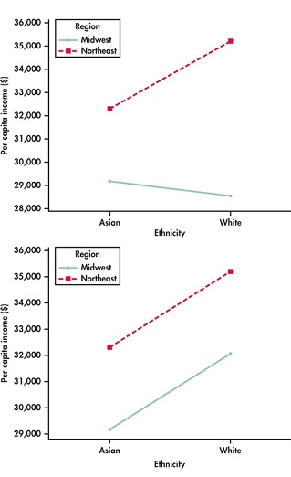
15-9

To examine two-way ANOVA data for a possible interaction, always construct a plot similar to Figure 15.1. Profiles that are roughly parallel imply that there is no clear interaction between the two factors. When no interaction is present, the marginal means provide a reasonable description of the two-way table of means.
In this case, it is clear that the two profiles (the collections of marginal means for a given region) are not parallel. When there is an interaction, the marginal means do not tell the whole story. For example, with these data, the marginal mean difference between regions is $4897. This is larger than the difference for Asian individuals ($3129) and smaller than the difference for white individuals ($6664).
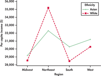
EXAMPLE 15.8 Per Capita Income, Continued
The American Community Survey in fact reports per capita income for four regions of the United States. Here are the data:
| Region | White | Asian | Mean |
| Midwest | $28,528 | $29,166 | $28,847 |
| Northeast | $35,192 | $32,295 | $33,744 |
| South | $28,455 | $30,246 | $29,351 |
| West | $30,264 | $31,176 | $30,720 |
| Mean | $30,610 | $30,721 | $30,665 |
Including the additional regions changes the marginal means for ethnicity and the overall mean of all groups. Figure 15.2 is a plot of the group means. There is a clear main effect for region: the per capita income of both white and Asian individuals is highest in the Northeast and West. The plot does not show a clear main effect for ethnicity because of the Northeast region. In all other regions, a person of Asian descent has a larger per capita income, but in the Northeast, the Asian per capita income is lower. As a result, the two lines are not parallel, indicating that an interaction is present. When there is interaction, main effects can be meaningful and important, but this is not always the case. For example, the main effect of region is meaningful despite the interaction, but the main effect of ethnicity is not as clear because of the interaction.
15-10
Apply Your Knowledge
Question 15.4
15.4 Marginal means.
Verify the marginal mean for Asian given in Example 15.8. Then verify that the overall mean at the lower-right of the table is the average of the two ethnicity means and also the average of the four region means.
Question 15.5
15.5 How do the differences depend on region?
One way to describe the interaction between region and ethnicity in Example 15.8 is to give the differences between the per capita income of individuals of white descent and individuals of Asian descent in the four regions. Plot the differences versus region, and write a short summary of what you conclude from the plot.
15.5
In the Northeast, the per capita income for white individuals is substantially higher than for Asian individuals; in the other 3 regions, the per capita income for Asian individuals is higher than for white individuals.
Question 15.6
15.6 Lack of interaction.
Suppose that the difference between the per capita income of white and Asian individuals remained fixed at $2897 for all four regions in Example 15.8 and that the per capita income for whites in each region is as given in the table. Find the per capita income for individuals of Asian descent in each region, and make a plot of the eight group means. In what important way does your plot differ from Figure 15.2?
Interactions come in many forms. When we find them, a careful examination of the means is needed to properly interpret the data. Simply stating that interactions are significant tells us little. Plots of the group means are very helpful.
EXAMPLE 15.9 Bundling as a Product Introduction Strategy
In Examples 15.3 and 15.4, we discussed a two-way design to investigate the effects of the partnered product’s brand image and complementarity on the new product’s perceived quality. Here are the means from a study that performed an experiment like this. The Sony brand name was used for the strong brand image, and the Haier brand name was used for the weak brand image.7 Figure 15.3 is the plot of the group means.
15-11
| Complementarity | |||
| Brand image | Low | High | Total |
| Low | 4.06 | 4.40 | 4.23 |
| High | 4.16 | 5.06 | 4.61 |
| Total | 4.11 | 4.73 | 4.42 |
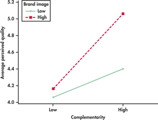
When the partnered product’s brand image is low, perceived quality of the surround sound receiver is about the same. When the brand image is high, the perceived quality increases regardless of complementarity. However, the perceived quality increases more when the partnered product’s complementarity is high (speaker system) than when it is low (camera).
In a statistical analysis, the pattern of means shown in Figure 15.3 produced significant main effects for brand image and complementarity in addition to a brand image–by–complementarity interaction. The main effects record that perceived quality is higher when the partnered product has high brand image and when the partnered product complements the new product. This clearly does not tell the whole story. We need to discuss the complementarity effect in each of the brand image levels to fully understand how perceived quality is affected.
A different kind of interaction is present in the next example. Here, we must be very cautious in our interpretation of the main effects as one of them can lead to a distorted conclusion.
EXAMPLE 15.10 Right Shade of Green
It is commonly thought that environmentally friendly consumption is driven by a desire to protect the environment and not to enhance one’s self-image. Is that the case in all settings? To study this, a two-factor experiment was run, in which subjects looked at an advertisement for a fuel-efficient vehicle and then reported their purchase intentions. One factor was whether the advertisement had a self-benefit or other-benefit appeal. The other factor was the type of accountability (public or private).8 Here are the mean purchase intentions:
15-12
| Accountability | |||
| Appeal | Public | Private | Mean |
| Self-benefit | 3.26 | 4.58 | 3.92 |
| Other-benefit | 4.84 | 3.37 | 4.11 |
| Mean | 4.05 | 3.98 | 4.01 |
The means are plotted in Figure 15.4. In the analysis of this experiment, only the interaction is statistically significant. How are we to interpret these results?
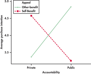
What catches our eye in the plot is that the lines cross. The purchase intention is much higher for the self-benefit advertisement in the private accountability condition, but the purchase intention was much higher for the other-benefit advertisement in the public accountability condition. This interaction between accountability and benefit is the important result. The main effects for accountability and appeal are not practically meaningful because of this interaction. Both factors have effects, but we must know which type of accountability a person is under in order to say which type of appeal results in higher purchase intent.
Apply Your Knowledge
Question 15.7
15.7 Is there an interaction?
Each of the following tables gives means for a two-way ANOVA. Make a plot of the means with the levels of Factor A on the x axis. State whether or not there is an interaction, and if there is, describe it.
Factor A Factor B 1 2 3 1 12 18 24 2 5 8 11 15-13
Factor A Factor B 1 2 3 1 10 15 20 2 30 35 40 Factor A Factor B 1 2 3 1 10 5 15 2 20 25 15 Factor A Factor B 1 2 3 1 20 5 20 2 10 25 10
15.7
(a) There is a slight interaction. Factor B level 1 is higher than Factor B level 2, but this difference increases as the level of Factor A increases, hence the interaction. (b) There is no interaction, Factor B level 2 is consistently higher than level 1 regardless of Factor A. Additionally, the means increase as Factor A level increases. (c) There is an interaction. For Factor A level 1, Factor B level 2 is higher than level 1; this difference increases for Factor A level 2. Finally there is no difference between level 2 and 1 for Factor B when Factor A is level 3. (d) There is an interaction, for Factor A levels 1 and 3, Factor B level 1 is higher than level 2; however, this reverses for Factor A level 2, where Factor B level 1 is now much higher than level 2.