CHAPTER 17 Review Exercises
For Exercises 17.1 and 17.2, see pages 17-3 to 17-4; for 17.3 and 17.4, see page 17-5; for 17.5 to 17.7, see page 17-8; for 17.8 to 17.10, see page 17-11; and for 17.11 to 17.13, see page 17-14.
Question 17.14
17.14 What's wrong?
For each of the following, explain what is wrong and why.
- For a multiple logistic regression with four explanatory variables, the null hypothesis that the regression coefficients of all the explanatory variables are zero is tested with an test.
- For a logistic regression we assume that the error term in our model has a Normal distribution.
- In logistic regression with two explanatory variables we use a chi-square statistic to test the null hypothesis versus a two-sided alternative.
17-18
Question 17.15
17.15 What's wrong?
For each of the following, explain what is wrong and why.
- If in a logistic regression analysis, we estimate that the probability of an event is multiplied by 2 when the value of the explanatory variable changes by 1.
- The intercept is equal to the odds of an event when .
- The odds of an event are 1 minus the probability of the event.
17.15
(a) It is not multiplied by 2. When the explanatory variable changes by 1, the odds are increased by a factor of e2 or 7.389 times. (b) It is missing the log; the intercept is equal to the log odds of an event when . (c) The odds of an event are the probability of the event divided by 1 minus the probability of the event.
Question 17.16
17.16 Is a movie profitable?
In Example 17.6 (pages 17-7 to 17-8), we developed a model to predict whether a movie will be profitable based on log opening-weekend revenue. What are the predicted odds of a movie being profitable if the opening-weekend revenue is
- $20 million dollars?
- $35 million dollars?
- $50 million dollars?
movprof
Question 17.17
17.17 Converting odds to probability.
Refer to the previous exercise. For each opening-weekend revenue, compute the estimated probability that the movie is profitable.
17.17
(a) 0.7170. (b) 0.7968. (c) 0.8383.
Question 17.18
17.18 Finding the best model?
In Example 17.11 (pages 17-16 to 17-7), we looked at a multiple logistic regression for movie profitability based on three explanatory variables. Complete the analysis by looking at the three models with two explanatory variable models and the three models with single variables. Create a table that includes the parameter estimates and their -values as well as the statistic and degrees of freedom. Based on the results, which model do you think is the best? Explain your answer.
movprof
Question 17.19
17.19 Tipping behavior in Canada.
The Consumer Report on Eating Share Trends (CREST) contains data that cover all provinces of Canada and that describe away-from-home food purchases by roughly 4000 households per quarter. Researchers recently restricted their attention to restaurants at which tips would normally be given.4 From a total of 73,822 observations, “high” and “low” tipping variables were created based on whether the observed tip rate was above 20% or below 10%, respectively. They then used logistic regression to identify explanatory variables associated with either “high” or “low” tips. Here is a table summarizing what they termed the stereotype-related variables for the high-tip analysis:
| Explanatory variable | Odds ratio |
| Senior adult | 0.7420* |
| Sunday | 0.9970 |
| English as second language | 0.7360* |
| French-speaking Canadian | 0.7840* |
| Alcoholic drinks | 1.1250* |
| Lone male | 1.0220 |
The starred odds ratios were significant at the 0.01 level. Write a short summary explaining these results in terms of the odds of leaving a high tip.
17.19
Those who order alcoholic drinks are 12.5% more likely (or 1.125 times as likely) to leave a high tip than those who don't order alcohol. Senior adults are about 25.8% less likely (or 0.742 times as likely) to leave a high tip than those who aren't senior. Those who speak English as a second language are about 26.4% less likely (or 0.736 times as likely) to leave a high tip than their counterparts. Those who are French-speaking Canadians are about 21.6% less likely (or 0.784 times as likely) to leave a high tip than those who aren't French-speaking Canadians.
Question 17.20
17.20 Sexual imagery in magazine ads.
In what ways do advertisers in magazines use sexual imagery to appeal to youth? One study classified each of 1509 full-page or larger ads as “not sexual” or “sexual,” according to the amount and style of the dress of the male or female model in the ad. The ads were also classified according to the target readership of the magazine.5 A logistic regression was used to describe the probability that the clothing in the ad was “not sexual” as a function of several explanatory variables. Here are some of the reported results:
| Explanatory variable | ||
| Reader age | 0.50 | 13.64 |
| Model sex | 1.31 | 72.15 |
| Men's magazines | −0.05 | 0.06 |
| Women's magazines | 0.45 | 6.44 |
| Constant | −2.32 | 135.92 |
Reader age is coded as 0 for young adult and 1 for mature adult. Therefore, the coefficient of 0.50 for this explanatory variable suggests that the probability that the model clothing is not sexual is higher when the target reader age is mature adult. In other words, the model clothing is more likely to be sexual when the target reader age is young adult. Model sex is coded as 0 for female and 1 for male. The explanatory variable men's magazines is 1 if the intended readership is men and 0 for women's magazines and magazines intended for both men and women (general interest). The variable women's magazines is coded similarly.
- State the null and alternative hypotheses for each of the explanatory variables.
- Perform the significance tests associated with the statistics.
- Interpret the sign of each of the statistically significant coefficients in terms of the probability that the model clothing is sexual.
- Write an equation for the fitted logistic regression model.
17-19
Question 17.21
17.21 Interpret the results.
Refer to the previous exercise. The researchers also reported odds ratios with 95% confidence intervals for this logistic regression model. Here is a summary:
| Explanatory variable |
95% confidence limits | ||
| Odds ratio | Lower | Upper | |
| Reader age | 1.65 | 1.27 | 2.16 |
| Model sex | 3.70 | 2.74 | 5.01 |
| Men's magazines | 0.96 | 0.67 | 1.37 |
| Women's magazines | 1.57 | 1.11 | 2.23 |
- Explain the relationship between the confidence intervals reported here and the results of the significance tests that you found in the previous exercise.
- Interpret the results in terms of the odds ratios.
- Write a short summary explaining the results. Include comments regarding the usefulness of the fitted coefficients versus the odds ratios in making a summary.
17.21
(a) If the confidence interval for the odds ratio includes the value 1, the variable is not significant in a logistic regression. (b) Because the Reader age, Model sex, and Women's magazines intervals all do not contain 1, they are all significant. The Men's magazine interval contains 1 and is not significant. (c) Interpreting only significant effects: When the reader age is mature adults, the model clothing is 1.27 to 2.16 times more likely to be not sexual. When the model sex is male, the model clothing is 2.74 to 5.01 times more likely to be not sexual. When the intended readership is women, the model clothing is 1.11 to 2.23 times more likely to be not sexual. The odds ratios are often much easier to interpret than the fitted coefficients.
Question 17.22
17.22 CEO overconfidence/dominance and corporate acquisitions.
The acquisition literature suggests that takeovers occur either due to conflicts between managers and shareholders or to create a new entity that exceeds the sum of its previously separate components. Other research has offered managerial hubris as a third option, but it has not been studied empirically. Recently, some researchers revisited acquisitions over a 10-year period in the Australian financial system.6 A measure of CEO overconfidence was based on the CEO's level of media exposure, and a measure of dominance was based on the CEO's remuneration relative to the firm's total assets. They then used logistic regression to see whether CEO overconfidence and dominance were positively related to the probability of at least one acquisition in a year. To help isolate the effects of CEO hubris, the model included explanatory variables of firm characteristics and other potentially important factors in the decision to acquire. The following table summarizes the results for the two key explanatory variables:
| Explanatory variable | ||
| Overconfidence | 0.0878 | 0.0402 |
| Dominance | 1.5067 | 0.0057 |
- State the null and alternative hypotheses for each of the explanatory variables.
- Perform the significance tests and determine whether the variables are significant at the 0.05 level.
- Estimate the odds ratio for each variable and construct a 95% confidence interval.
- Write a short summary explaining the results.
Question 17.23
17.23 E-government use in Canada.
Electronic government (e-government) provides digital means, such as an email address or a website, for citizens to contact public officials. The vision behind e-government is to create a more citizen-focused government. One study used survey data to determine what factors are related to a citizen using an e-government website rather than visiting or calling a government office.7 The dependent variable refers to whether the citizen used the website or not. Explanatory variables include sex (1 = female, 0 =male), daily Internet use (1 = yes, 0=no), age (six ordered categories numbered 1 through 6), household income (seven ordered categories numbered 1 through 7), size of the community (six ordered categories numbered 1 through 6), and education (1 = at least some postsecondary education, 0 = other). The following table summarizes the results.
| Explanatory variable | Odds ratio |
| Sex | 0.87 |
| Daily Internet use | 4.16 |
| Age | 0.81 |
| Income | 1.01 |
| Size | 0.85 |
| Education | 0.97 |
| Intercept | 0.66 |
All but “Education” and “Income” were significant at the 0.05 level.
- Interpret each of the odds ratios in terms of the probability that the individual uses the website.
- Compute the regression coefficients for each of the variables in the table.
- What are the odds that a male college graduate, who uses the Internet daily, is age category 3, household Income level 4, and community size 5 is using the Internet?
17.23
(a) Females are 0.87 times as likely (13% less likely) to use the website as males. Daily Internet users are 4.16 times as likely to use the website as their counterparts. Older-aged people are less likely to use the website than younger-aged people. Those from larger communities are less likely to use the website than those from smaller communities. Those with different incomes and/or educations are about equally likely to use the website because they aren't significantly different from 1. (b) , Daily Internet use: 1.4255, , Income: 0.01, , , . (c) 0.6537.
Question 17.24
17.24 Business Travel.
The Best Western Small Business Travel survey reported that 355 of 400 U.S. small business owners plan as many business trips this fall as last year.8
- What proportion of U.S. small business owners plan as many trips as last year?
- What are the odds that an owner will say that his or her company plans as many business trips as last year?
- What proportion of owners said that they do not plan as many trips this year?
- What are the odds that an owner will say that they are cutting back on business trips this year?
- How are your answers to parts (b) and (d) related?
17-20
Question 17.25
17.25 Stock options.
Different kinds of companies compensate their key employees in different ways. Established companies may pay higher salaries, while new companies may offer stock options that will be valuable if the company succeeds. Do high-tech companies tend to offer stock options more often than other companies? One study looked at a random sample of 200 companies. Of these, 91 were listed in the Directory of Public High Technology Corporations, and 109 were not listed. Treat these two groups as SRSs of high-tech and non-high-tech companies. Seventy-three of the high-tech companies and 75 of the non-high-tech companies offered incentive stock options to key employees.9
- What proportion of the high-tech companies offer stock options to their key employees? What are the odds?
- What proportion of the non-high-tech companies offer stock options to their key employees? What are the odds?
- Find the odds ratio using the odds for the high-tech companies in the numerator. Interpret the result in a few sentences.
17.25
(a) 0.8022. . (b) 0.6881. . (c) odds . The high-tech companies are 1.8385 times more likely to offer incentive stock options to key employees than the non-high-tech companies.
Question 17.26
17.26 Log odds for high-tech and non-high-tech firms.
Refer to the previous exercise.
- Find the log odds for the high-tech firms. Do the same for the non-high-tech firms.
- Define an explanatory variable to have the value 1 for high-tech firms and 0 for non-high-tech firms. For the logistic model, we set the log odds equal to . Find the estimates and for the parameters and .
- Show that the odds ratio is equal to
Question 17.27
17.27 Do the inference.
Refer to the previous exercise. Software gives 0.3347 for the standard error of .
- Find the 95% confidence interval for .
- Transform your interval in (a) to a 95% confidence interval for the odds ratio.
- What do you conclude?
17.27
(a) (–0.047, 1.265). (b) (0.954, 3.543). (c) Because the interval in part (b) includes 1, there is no significant difference in the proportions of high-tech and non-high-tech companies that offer stock options to key employees.
Question 17.28
17.28 Suppose you had twice as many data.
Refer to Exercises 17.25 through 17.27. Repeat the calculations assuming that you have twice as many observations with the same proportions. In other words, assume that there are 182 high-tech firms and 218 non-high-tech firms. The numbers of firms offering stock options are 146 for the high-tech group and 150 for the non-high-tech group. The standard error of for this scenario is 0.2366. Summarize your results, paying particular attention to what remains the same and what is different from what you found in Exercises 17.25 through 17.27.
Question 17.29
17.29 Poor service.
In the food service industry, some argue tipping encourages servers to provide discriminate service. If the server expects a good tip, he or she may provide better service. In one survey, 193 servers were surveyed and asked if they ever provided poor service because they did not expect a good tip. Ninety-six replied yes.10
- What proportion of the servers have provided poor service because of an expected bad tip?
- What are the odds that a server will have provided bad service given an expected bad tip?
- What proportion of the servers did not provide bad service?
- What are the odds that a server will not have provided bad service ?
- How are your answers to parts (b) and (d) related?
17.29
(a) 0.4974. (b) . (c) 0.5026. (d) . (e) They are reciprocals.
Question 17.30
17.30 Active retail companies versus failed companies.
Case 7.2 (page 389) compared the cash flow of 74 active retail firms with the cash flow for 27 firms that failed. Here we analyze the same data with a logistic regression. The outcome is whether or not the firm is active, and the explanatory variable is the cash flow. Here is the output from Minitab:
cmps
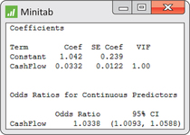
- Give the fitted equation for the log odds that a firm will be active.
- Describe the results of the significance test for the coefficient of cash flow.
- The odds ratio is the estimated amount that the odds of being active would increase when the cash flow is increased by one unit. Report this odds ratio with the 95% confidence interval.
- Write a short summary of this analysis and compare it with the analysis of these data that we performed in Chapter 7. Which approach do you prefer?
17-21
Question 17.31
17.31 Analysis of a reduction in force.
To meet competition or cope with economic slowdowns, corporations sometimes undertake a “reduction in force” (RIF), in which substantial numbers of employees are terminated. Federal and various state laws require that employees be treated equally regardless of their age. In particular, employees over the age of 40 years are in a “protected” class, and many allegations of discrimination focus on comparing employees over 40 with their younger coworkers. Here are the data for a recent RIF:
| Over 40 | ||
| Terminated | No | Yes |
| Yes | 17 | 71 |
| No | 564 | 835 |
- Write the logistic regression model for this problem using the log odds of a termination as the response variable and an indicator for over and under 40 years of age as the explanatory variable.
- Explain the assumption concerning binomial distributions in terms of the variables in this exercise. To what extent do you think that these assumptions are reasonable?
- Software gives the estimated slope and its standard error . Transform the results to the odds scale. Summarize the results and write a short conclusion.
- If additional explanatory variables were available, for example, a performance evaluation, how would you use this information to study the RIF?
17.31
(a) . (b) The binomial distribution assumes that each employee's termination is independent from one another's and the probability of being terminated is the same for each employee. Certainly the latter is not true because an individual's performance is likely different and largely determines whether or not they are terminated. (c) , with 95% the confidence interval is (1.644, 4.840). Because the interval does not contain 1, the results are significant at the 5% level. Employees over 40 are 2.82 times more likely to be terminated than those under 40. (d) We could use the additional variables in the logistic regression model to account for their effects before assessing if age has an effect.
Question 17.32
17.32 Following brands through social media.
PricewaterhouseCoopers (PwC) surveyed 1000 online shoppers in the United States and China.11 One question asked if the online shopper followed brands they purchased through social media. Here are the results:
| Social media | ||
| Country | No | Yes |
| United States | 487 | 513 |
| China | 72 | 928 |
- What are the proportions of online shoppers who follow brands through social media in each country?
- What is the odds ratio for comparing U.S. online shoppers with Chinese online shoppers?
- Write the logistic regression model for this problem using the log odds of following brands through social media as the response variable and country as an indicator explanatory variable .
- Software gives the estimated slope and its standard error . Transform this result to the odds scale and compare it with your answer in part (b).
- Construct a 95% confidence interval for the odds ratio and write a short conclusion.
Question 17.33
17.33 Know your customers.
To devise effective marketing strategies, it is helpful to know the characteristics of your customers. A study compared demographic characteristics of people who use the Internet for travel arrangements and of people who do not.12 Of 1132 Internet users, 643 had completed college. Among the 852 nonusers, 349 had completed college. Model the log odds of using the Internet to make travel arrangements with an indicator variable for having completed college as the explanatory variable. Summarize your findings.
17.33
. , . The odds ratio estimate is 1.8952; that is, those who have completed college are 1.8952 times more likely to use the Internet for travel arrangements than those who have not completed college.
Question 17.34
17.34 Does income relate to use of the Internet?
The study mentioned in the previous exercise also asked about income. Among Internet users, 493 reported income of less than $50,000, and 378 reported income of $50,000 or more. (Not everyone answered the income question.) The corresponding numbers for nonusers were 477 and 200. Repeat the analysis using an indicator variable for income of $50,000 or more as the explanatory variable. What do you conclude?
For the following five exercises, you will need to construct indicator variables to use categorical variables as explanatory variables in logistic regression. Be sure to review the material in Chapter 11 on models with categorical explanatory variables (pages 571-575) before attempting these exercises.
Question 17.35
17.35 Reduction in force using logistic regression.
In Exercise 17.31, hypothetical data are given for a reduction in force (RIF). If there is a statistically significant difference in the RIF proportions based on age group, the employer needs to justify the difference based on other (nondiscriminatory) variables.
rif
- Run the logistic analysis to predict the odds of being riffed using age group (over 40 years of age or not) as the explanatory variable. Summarize your results.
- What other variables would you add to the model in an attempt to explain the results that you described in part (a)? If these other variables can be shown to be characteristics that relate to job performance, and the age effect is no longer significant in a model that includes these variables, then the analysis provides statistical evidence that can be used to refute a claim of discrimination.
17.35
(a) The model is significant. For a person over 40: 0.085. For a person under 40: 0.030. (b) Answers will vary.
17-22
Question 17.36
17.36 Sexual imagery in ads.
Refer to Exercise 17.20 (page 17-18) concerning the use of sexual imagery in magazine ads. Here is the two-way table of counts for the 1509 ads.
| Magazine readership | ||||
| Model dress | Women | Men | General interest | Total |
| Not sexual | 351 | 514 | 248 | 1113 |
| Sexual | 225 | 105 | 66 | 396 |
| Total | 576 | 619 | 314 | 1509 |
Use the model dress, expressed as the odds that the dress is sexual, as the response variable and the magazine readership as the explanatory variable. Because there are three magazine readership categories, you will need two indicator variables for this multiple logistic regression analysis. Use the last category, general interest, for the “other” designation when creating these indicator variables.
imagery
- A friend has suggested that the three magazine categories be coded as 1, 2, 3 and that this single variable be used as the explanatory variable in the logistic regression. Explain why this analytical strategy is wrong.
- Summarize the results of the significance testing. Do the data support the idea that the sexual content expressed in the model dress varies by the magazine readership?
- Use the estimates for your model and the coding that you used for the explanatory variables to give the estimated log odds for each type of magazine readership.
Question 17.37
17.37 Rerun the analysis with a different coding.
In the previous exercise, you used the last category, general interest, for the “other” designation when you constructed the indicator variables. Now use the women's magazine readership as the “other” category and reanalyze the data. Verify that the significance testing results for the effect of the two explanatory variables is the same as in the previous exercise.
imagery
17.37
The estimated model becomes
Now both men
and general terms are significant.
Question 17.38
17.38 Student athletes and gambling.
A survey of student athletes that asked questions about gambling behavior classified students according to the National Collegiate Athletic Association (NCAA) division.13 For male student athletes, the percent who reported wagering on collegiate sports are given here along with the numbers of respondents in each division:
| Division | |||
| I | II | III | |
| Percent | 17.2% | 21.0% | 24.4% |
| Number | 5619 | 2957 | 4089 |
- Using the numbers and percents given, calculate the numbers of students who gamble and those who do not for each NCAA division.
- Use two indicator variables to code the explanatory variable, NCAA division. Let the first one be 1 for Division II and 0 otherwise; let the second be 1 for Division III and 0 otherwise. With this coding, the logistic regression model will use the intercept for Division I, the intercept plus the coefficient of the first indicator variable for Division II, and the intercept plus the coefficient of the second indicator variable for Division III.
- Run the multiple logistic regression and summarize the results.
Question 17.39
17.39 Is there a trend?
Refer to the previous exercise. The coding of the indicator variables suggests a way to code models when you expect a pattern in the response that is based on some kind of ordering of the explanatory variable. In some settings this is called detecting a dose response.
- Use the model to give the estimated log odds for each NCAA division.
- Plot these estimates versus division and summarize the results. Does there appear to be a pattern in the results?
- How would you model the pattern that you described in part (b)?
17.39
(a) For Division . For Division . For Division . (b) The plot shows that log(odds) of gambling increases as Division increases. (c) Because the relationship is quite linear, we could use a regression analysis.