Section 1.4 Exercises
For Exercise 1.70, see page 40; for 1.71 to 1.73, see pages 41-42; for 1.74 to 1.77, see pages 44-45; for 1.78, see page 46; for 1.79 and 1.80, see page 49; for 1.81 and 1.82, see page 50; and for 1.83 and 1.84, see page 53.
Question 1.85
1.85 Find the error.
Each of the following statements contains an error. Describe the error and then correct the statement.
- A density curve is a mathematical model for the distribution of a categorical variable.
- The area under the curve for a density curve is always greater than the mean.
- If a variable can take only negative values, then the density curve for its distribution will lie entirely below the x axis.
1.85
(a) A density curve is a mathematical model for the distribution of a quantitative variable. (b) The area under the curve for a density curve is always equal to 1. (c) If a variable can take only negative values, then the density curve for its distribution will still lie entirely above the axis.
Question 1.86
1.86 Find the error.
Each of the following statements contains an error. Describe the error and then correct the statement.
- The 68-95-99.7 rule applies to all distributions.
- A normal distribution can take only positive values.
- For a symmetric distribution, the mean will be larger than the median.
Question 1.87
1.87 Sketch some Normal curves.
- Sketch a Normal curve that has mean 30 and standard deviation 4.
- On the same x axis, sketch a Normal curve that has mean 20 and standard deviation 4.
- How does the Normal curve change when the mean is varied but the standard deviation stays the same?
1.87
(c) The curve shifts to the left or right, but the spread remains the same.
Question 1.88
1.88 The effect of changing the standard deviation.
- Sketch a Normal curve that has mean 20 and standard deviation 5.
- On the same x axis, sketch a Normal curve that has mean 20 and standard deviation 2.
- How does the Normal curve change when the standard deviation is varied but the mean stays the same?
Question 1.89
1.89 Know your density.
Sketch density curves that might describe distributions with the following shapes.
- Symmetric, but with two peaks (that is, two strong clusters of observations).
- Single peak and skewed to the left.
Question 1.90
1.90 Gross domestic product.
Refer to Exercise 1.46, where we examined the gross domestic product of 189 countries.
gdp
- Compute the mean and the standard deviation.
- Apply the 68-95-99.7 rule to this distribution.
- Compare the results of the rule with the actual percents within one, two, and three standard deviations of the mean.
- Summarize your conclusions.
Question 1.91
1.91 Do women talk more?
Conventional wisdom suggests that women are more talkative than men. One study designed to examine this stereotype collected data on the speech of 42 women and 37 men in the United States.30
- The mean number of words spoken per day by the women was 14,297 with a standard deviation of 9065. Use the 68-95-99.7 rule to describe this distribution.
- Do you think that applying the rule in this situation is reasonable? Explain your answer.
- The men averaged 14,060 words per day with a standard deviation of 9056. Answer the questions in parts (a) and (b) for the men.
- Do you think that the data support the conventional wisdom? Explain your answer. Note that in Section 7.2, we will learn formal statistical methods to answer this type of question.
1.91
(a) According to the rule, 68% of women speak between 5232 and 23,362 words per day, 95% of women speak between -3833 and 32,427 words per day, and 99.7% of women speak between -12,898 and 41,492 words per day. (b) This rule doesn—t seem to fit because you can—t speak a negative amount of words per day; therefore, the percentages don—t make sense. (c) According to the rule, 68% of men speak between 5004 and 23,116 words per day, 95% of men speak between -4052 and 32,172 words per day, and 99.7% of men speak between -13,108 and 41,228 words per day. Similar to the women, the rule doesn—t seem to fit because, again, you can—t speak a negative amount of words per day, so the percentages don—t make sense. (d) The data do show that the mean number of words spoken per day is higher for women than for men, but it is very close; in addition, the standard deviations are nearly the same, making the intervals very close. To put it in perspective, the women only speak about 1-2% more words per day on average. That small of a difference could just be due to chance.
58
Question 1.92
1.92 Data from Mexico.
Refer to the previous exercise. A similar study in Mexico was conducted with 31 women and 20 men. The women averaged 14,704 words per day with a standard deviation of 6215. For men, the mean was 15,022 and the standard deviation was 7864.
- Answer the questions from the previous exercise for the Mexican study.
- The means for both men and women are higher for the Mexican study than for the U.S. study. What conclusions can you draw from this observation?
Question 1.93
1.93 Total scores for accounting course.
Following are the total scores of 10 students in an accounting course:
acct
| 62 | 93 | 54 | 76 | 73 | 98 | 64 | 55 | 80 | 71 |
Previous experience with this course suggests that these scores should come from a distribution that is approximately Normal with mean 72 and standard deviation 10.
- Using these values for and , standardize the scores of these 10 students.
- If the grading policy is to give a grade of A to the top 15% of scores based on the Normal distribution with mean 72 and standard deviation 10, what is the cutoff for an A in terms of a standardized score?
- Which students earned an A for this course?
1.93
(a) The standardized values are: -1, 2.1, -1.8, 0.4, 0.1, 2.6, -0.8, -1.7, 0.8, -0.1. (b) 85 percentile ? . (c) Only two scores, the 93 and the 98.
Question 1.94
1.94 Assign more grades.
acct
Refer to the previous exercise. The grading policy says that the cutoffs for the other grades correspond to the following: the bottom 5% receive an F, the next 15% receive a D, the next 35% receive a C, and the next 30% receive a B. These cutoffs are based on the distribution.
- Give the cutoffs for the grades in terms of standardized scores.
- Give the cutoffs in terms of actual scores.
- Do you think that this method of assigning grades is a good one? Give reasons for your answer.
Question 1.95
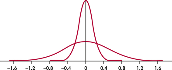
1.95 Visualizing the standard deviation.
Figure 1.34 shows two Normal curves, both with mean 0. Approximately what is the standard deviation of each of these curves?
1.95
The wider curve has a standard deviation of about 0.4. The narrower curve has a standard deviation about 0.2.
Question 1.96
1.96 Exploring Normal quantile plots.
- Create three data sets: one that is clearly skewed to the right, one that is clearly skewed to the left, and one that is clearly symmetric and mound-shaped. (As an alternative to creating data sets, you can look through this chapter and find an example of each type of data set requested.)
- Using statistical software, obtain Normal quantile plots for each of your three data sets.
- Clearly describe the pattern of each data set in the Normal quantile plots from part (b).
Question 1.97
1.97 Length of pregnancies.
The length of human pregnancies from conception to birth varies according to a distribution that is approximately Normal with mean 266 days and standard deviation 16 days. Use the 68-95-99.7 rule to answer the following questions.
- Between what values do the lengths of the middle 95% of all pregnancies fall?
- How short are the shortest 2.5% of all pregnancies?
1.97
(a) 95% of pregnancies last between 234 and 298 days. (b) The shortest pregnancies are 234 days or less.
Question 1.98
1.98 Uniform random numbers.
Use software to generate 100 observations from the distribution described in Exercise 1.72 (page 41). (The software will probably call this a “uniform distribution.”) Make a histogram of these observations. How does the histogram compare with the density curve in Figure 1.20? Make a Normal quantile plot of your data. According to this plot, how does the uniform distribution deviate from Normality?
Question 1.99
1.99 Use Table A or software.
Use Table A or software to find the proportion of observations from a standard Normal distribution that falls in each of the following regions. In each case, sketch a standard Normal curve and shade the area representing the region.
1.99
(a) 0.0179. (b) 0.9821. (c) 0.0548. (d) 0.9273.
59
Question 1.100
1.100 Use Table A or software.
Use Table A or software to find the value of for each of the following situations. In each case, sketch a standard Normal curve and shade the area representing the region.
- Twelve percent of the values of a standard Normal distribution are greater than .
- Twelve percent of the values of a standard Normal distribution are greater than or equal to .
- Twelve percent of the values of a standard Normal distribution are less than .
- Fifty percent of the values of a standard Normal distribution are less than .
Question 1.101
1.101 Use Table A or software.
Consider a Normal distribution with mean 200 and standard deviation 20.
- Find the proportion of the distribution with values between 190 and 220. Illustrate your calculation with a sketch.
- Find the value of such that the proportion of the distribution with values between and is 0.75. Illustrate your calculation with a sketch.
1.101
(a) Between -0.5 and 1. 0.5328. (b) corresponds with the 12.5 percentile . corresponds with the 87.5 percentile . Solving gives .
Question 1.102
1.102 Length of pregnancies.
The length of human pregnancies from conception to birth varies according to a distribution that is approximately Normal with mean 266 days and standard deviation 16 days.
- What percent of pregnancies last fewer than 240 days (that is, about 8 months)?
- What percent of pregnancies last between 240 and 270 days (roughly between 8 and 9 months)?
- How long do the longest 20% of pregnancies last?
Question 1.103
1.103 Quartiles of Normal distributions.
The median of any Normal distribution is the same as its mean. We can use Normal calculations to find the quartiles for Normal distributions.
- What is the area under the standard Normal curve to the left of the first quartile? Use this to find the value of the first quartile for a standard Normal distribution. Find the third quartile similarly.
- Your work in part (a) gives the Normal scores for the quartiles of any Normal distribution. What are the quartiles for the lengths of human pregnancies? (Use the distribution given in the previous exercise.)
1.103
(a) The area to the left of the first quartile is 25%. The corresponding is -0.67. The area to the left of the third quartile is 75%. The corresponding is 0.67. (b) For the first quartile, . For the third quartile, .
Question 1.104
1.104 Deciles of Normal distributions.
The deciles of any distribution are the 10th, 20th, . . . , 90th percentiles. The first and last deciles are the 10th and 90th percentiles, respectively.
- What are the first and last deciles of the standard Normal distribution?
- The weights of 9-ounce potato chip bags are approximately Normal with a mean of 9.12 ounces and a standard deviation of 0.15 ounce. What are the first and last deciles of this distribution?
Question 1.105
1.105 Normal random numbers.
Use software to generate 100 observations from the standard Normal distribution. Make a histogram of these observations. How does the shape of the histogram compare with a Normal density curve? Make a Normal quantile plot of the data. Does the plot suggest any important deviations from Normality? (Repeating this exercise several times is a good way to become familiar with how Normal quantile plots look when data are actually close to Normal.)
1.105
(a) For those who get enough sleep, 56.8% are high exercisers and 43.2% are low exercisers. (b) For those who don't get enough sleep, 37.9% are high exercisers and 62.1% are low exercisers. (c) Those who get enough sleep are more likely to be high exercisers than those who don't get enough sleep.
Question 1.106
1.106 Trade balance.
bestbus
Refer to Exercise 1.49 (page 35) where you examined the distribution of trade balance for 145 countries in the best countries for business data set. Generate a histogram and a normal quantile plot for these data. Describe the shape of the distribution and whether or not the normal quantile plot suggests that this distribution is Normal.
Question 1.107
1.107 Gross domestic product per capita.
Refer to the previous exercise. The data set also contains the gross domestic product per capita calculated by dividing the gross domestic produce by the size of the population for each country.
bestbus
- Generate a histogram and a normal quantile plot for these data.
- Describe the shape of the distribution and whether or not the normal quantile plot suggests that this distribution is Normal.
- Explain why GDP per capita might be a better variable to use than GDP for assessing how favorable a country is for business.
1.107
(b) The distribution is right-skewed; this is also shown in the Normal quantile plot.