5.2 The Poisson Distributions
A count has a binomial distribution when it is produced under the binomial setting. If one or more facets of this setting do not hold, the count will have a different distribution. In this section, we discuss one of these distributions.
Frequently, we meet counts that are open-ended (that is, are not based on a fixed number of observations): the number of customers at a popular café between 12:00 P.M. and 1:00 P.M.; the number of finish defects in the sheet metal of a car; the number of workplace injuries during a given month; the number of impurities in a liter of water. These are all counts that could be 0, 1, 2, 3, and so on indefinitely. Recall from Chapter 4 that when count values potentially go on indefinitely, they are said to be countably infinite.
Reminder

countably infinite, p. 210
The Poisson setting
The Poisson distribution is another model for a count and can often be used in these open-ended situations. The count represents the number of events (call them “successes”) that occur in some fixed unit of measure such as a interval of time, region of area, or region of space. The Poisson distribution is appropriate under the following conditions.
The Poisson Setting
- The number of successes that occur in two nonoverlapping units of measure are independent.
- The probability that a success will occur in a unit of measure is the same for all units of equal size and is proportional to the size of the unit.
- The probability that more than one event occurs in a unit of measure is negligible for very small-sized units. In other words, the events occur one at a time.
268
For binomial distributions, the important quantities were , the fixed number of observations, and , the probability of success on any given observation. For Poisson distributions, the only important quantity is the mean number of successes occurring per unit of measure.
Poisson Distribution
The distribution of the count of successes in the Poisson setting is the Poisson distribution with mean . The parameter is the mean number of successes per unit of measure. The possible values of are the whole numbers 0, 1, 2, 3, .... If is any whole number, then*
The standard deviation of the distribution is .
EXAMPLE 5.16 Number of Wi-Fi Interruptions
Suppose that the number of wi-fi interruptions on your home network varies, with an average of 0.9 interruption per day. If we assume that the Poisson setting is reasonable for this situation, we can model the daily count of interruptions using the Poisson distribution with . What is the probability of having no more than two interruptions tomorrow?
We can calculate either using software or the Poisson probability formula. Using the probability formula:
Using Excel, we can use the “POISSON.DIST()” function to find the individual probabilities. The function has three arguments. The first argument is the value of , the second argument is the mean value , and the third argument is the value “0,” which tells Excel to report an individual probability. For example, we put the entry of “= POISSON.DIST(2, 0.9, 0)” to obtain . Here is a summary of the calculations using Excel:
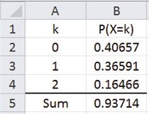
The reported value of 0.93714 was obtained by using Excel’s SUM function. Excel’s answer and the preceding hand-computed answer differ slightly due to roundoff error in the hand calculation. There is roughly a 94% chance that you will have no more than two wi-fi interruptions tomorrow.
*The in the Poisson probability formula is a mathematical constant equal to 2.71828 to five decimal places. Many calculators have an function.
269
Similar to the binomial, Poisson probability calculations are rarely done by hand if the event includes numerous possible values for . Most software provides functions to calculate and the cumulative probabilities of the form . These cumulative probability calculations make solving many problems less tedious. Here’s an example.
EXAMPLE 5.17 Counting ATM Customers
Suppose the number of persons using an ATM in any given hour between 9 A.M. and 5 P.M. can be modeled by a Poisson distribution with . What is the probability that more than 10 persons will use the machine between 3 P.M. and 4 P.M.?
Calculating this probability requires two steps:
- Write as an expression involving a cumulative probability:
- Calculate and subtract the value from 1. Using Excel, we again employ the “POISSON.DIST()” function. However, the third argument in the function should be “1,” which tells Excel to report a cumulative probability. Thus, we put the entry of “=POISSON.DIST(10, 8.5, 1)” to obtain . Here is a summary in Excel:
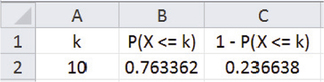
The probability that more than 10 persons will use the ATM between 3 P.M. and 4 P.M. is about 0.24. Relying on software to get the cumulative probability is much quicker and less prone to error than the method of Example 5.16 (page 268). For this case, that method would involve determining 11 probabilities and then summing their values.
Under the Poisson setting, this probability of 0.24 applies not only to the 3–4 P.M. hour but to any hour during the day period of 9 A.M. to 5 P.M.
Apply Your Knowledge
Question 5.40
5.40 ATM customers.
Refer to Example 5.17. Use the Poisson model to compute the probability that four or fewer customers will use the ATM machine during any given hour between 9 A.M. and 5 P.M.
Question 5.41
5.41 Number of wi-fi interruptions.
Refer to Example 5.16. What is the probability of having at least one wi-fi interruption on any given day?
5.41
0.5934.
The Poisson model
If we add counts from two nonoverlapping areas, we are just counting the successes in a larger area. That count still meets the conditions of the Poisson setting. If the individual areas were equal in size, our unit of measure doubles, resulting in the mean of the new count being twice as large. In general, if is a Poisson random variable with mean and is a Poisson random variable with mean and is independent of , then is a Poisson random variable with mean This fact means that we can combine areas or look at a portion of an area and still use Poisson distributions to model the count.
270
EXAMPLE 5.18 Paint Finish Flaws

Auto bodies are painted during manufacture by robots programmed to move in such a way that the paint is uniform in thickness and quality. You are testing a newly programmed robot by counting paint sags caused by small areas receiving too much paint. Sags are more common on vertical surfaces. Suppose that counts of sags on the roof follow the Poisson model with mean 0.7 sag per square yard and that counts on the side panels of the auto body follow the Poisson model with mean 1.4 sags per square yard. Counts in nonoverlapping areas are independent. Then
- The number of sags in two square yards of roof is a Poisson random variable with mean .
- The total roof area of the auto body is 4.8 square yards. The number of paint sags on a roof is a Poisson random variable with mean .
- A square foot is 1/9 square yard. The number of paint sags in a square foot of roof is a Poisson random variable with mean .
- If we examine one square yard of roof and one square yard of side panel, the number of sags is a Poisson random variable with mean .
Approximations to the Poisson
When the mean of the Poisson distribution is large, it may be difficult to calculate Poisson probabilities using a calculator. Fortunately, when is large, Poisson probabilities can be approximated using the Normal distribution with mean and standard deviation Here is an example.
EXAMPLE 5.19 Number of Text Messages Sent
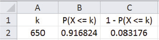
Americans aged 18 to 29 years send an average of almost 88 text messages a day.11 Suppose that the number of text messages you send per day follows a Poisson distribution with mean 88. What is the probability that over a week you would send more than 650 text messages?
To answer this using software, we first compute the mean number of text messages sent per week. Since there are seven days in a week, the mean is . Using Excel tells us that there is slightly more than an 8% chance of sending this many texts:
For the Normal approximation, we compute
The approximation is quite accurate, differing from the actual probability by only 0.0021.
271
While the Normal approximation is adequate for many practical purposes, were commend using statistical software when possible so you can get exact Poisson probabilities.
There is one other approximation associated with the Poisson distribution that is worth mentioning. It is related to the binomial distribution. Previously, we recommended using the Normal distribution to approximate the binomial distribution when and satisfy and . In cases where is large but is so small that , the Poisson distribution with yields more accurate results. For example, suppose that you wanted to calculate when has the distribution. Using Excel, we can employ the “BINOM.DIST()” function to find binomial probabilities. Here are the actual binomial probability and the Poisson approximation as reported by Excel
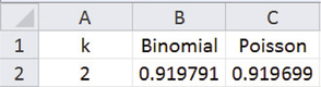
The Poisson approximation gives a very accurate probability calculation for the binomial distribution in this case.
Apply Your Knowledge
Question 5.42
5.42 Industrial accidents.
A large manufacturing plant has averaged seven “reportable accidents” per month. Suppose that accident counts over time follow a Poisson distribution with mean seven per month.
- What is the probability of exactly seven accidents in a month?
- What is the probability of seven or fewer accidents in a month?
Question 5.43
5.43 A safety initiative.
This year, a “safety culture change” initiative attempts to reduce the number of accidents at the plant described in the previous exercise. There are 60 reportable accidents during the year. Suppose that the Poisson distribution of the previous exercise continues to apply.
- What is the distribution of the number of reportable accidents in a year?
- What is the probability of 60 or fewer accidents in a year? (Use software.)
Does the computed probability suggest that there is evidence that the initiative did reduce the accident rate? Explain why or why not.
5.43
(a) Poisson with (b) 0.00367. Yes, because the probability is so small, it is unlikely to have occurred by chance; the initiative seems to have reduced the accident rate.
Assessing Poisson assumption with data
Similar to the binomial distribution, the applicability of Poisson distribution requires that certain specific conditions are met. In particular, we model counts with the Poisson distribution if we are confident that the counts arise from a Poisson setting (page 267). Let’s consider a couple of examples to see if the Poisson model reasonably applies.
EXAMPLE 5.20 English Premier League Goals
epl
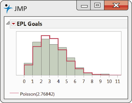
Consider data on the total number of goals scored per soccer game in the English Premier League (EPL) for the 2013–2014 regular season.12 Over the 380 games played in the season, the average number of goals per game is 2.768.
The Poisson distribution has a unique characteristic in that the standard deviation of the Poisson random variable is equal to the square root of the mean. In turn, this implies that the mean of a Poisson random variable equals its variance; that is, . This fact provides us with a very convenient quick check for Poisson compatibility—namely, compare the mean observed count with the observed variance. For the goal data, we find the sample variance of the counts to be 3.002, which is quite close to the mean of 2.768. This suggests that the Poisson distribution might serve a reasonable model for counts on EPL goals per game.
272
Figure 5.10 shows a JMP-produced graph of a Poisson distribution with overlaid on the count data. The Poisson distribution and observed counts show quite a good match. It would be reasonable to assume that the variability in goals scored in EPL games is well acounted by the Poisson distribution.
The next example shows a different story.
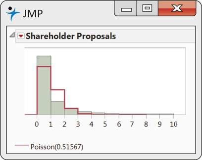
EXAMPLE 5.21 Shareholder Proposals
The U.S. Securities and Exchange Commission (SEC) entitles shareowners of a public company who own at least $2000 in market values of a company’s outstanding stock to submit shareholder proposals. A shareholder proposal is a resolution put forward by a shareholder, or group of shareholders, to be voted on at the company’s annual meeting. Shareholder proposals serve as a means for investor activists to effect change on corporate governance and activities. Proposals can range from executive compensation to corporate social responsibility issues, such as human rights, labor relations, and global warming. The SEC requires companies to disclose shareholder proposals on the company’s proxy statement. Proxy statements are publicly available.
In a study of 1532 companies, data were gathered on the counts of shareholder proposals per year.13 The mean number of shareholder proposals can be found to be 0.5157 per year. We would find that observed variance of the counts is 1.1748, which is more than twice the mean value. This implies that the counts are varying to a greater degree than expected by the Poisson model. As noted with Example 5.15 (page 262), this phenomenon is known as overdispersion. Figure 5.11 shows a JMP produced graph of a Poisson distribution with overlaid on the count data. The figure shows the incompatibility of the Poisson model with the observed count data. We find that there are more zero counts than expected, along with more higher counts than expected.
The extra abundance of zeroes in the count data of Example 5.21 is known as a zero inflation phenomenon. Researchers of this study hypothesize that the increased count of zeroes is due to many companies choosing to privately resolve shareholder concerns so as to protect their corporate image. In the end, the Poisson distribution does not serve as an appropriate model for the counts of shareholder proposals.
zero inflation
273