6.1 The Sampling Distribution of a Sample Mean
Suppose that you plan to survey 1000 students at your university about their sleeping habits. The sampling distribution of the average hours of sleep per night describes what this average would be if many simple random samples (SRSs) of 1000 students were drawn from the population of students at your university. In other words, it gives you an idea of what you are likely to see from your survey. It tells you whether you should expect this average to be near the population mean and whether the variation of the statistic is roughly ±2 hours or ±2 minutes.
To help in the transition from probability as a topic in itself to probability as a foundation for inference, in this chapter we carefully study the sampling distribution of and describe how it is used in inference when the data are from a large population with known standard deviation . In later chapters, we address the sampling distributions of other statistics more commonly used in inference. The reason we focus on just this one case here is because the general framework for constructing and using a sampling distribution for inference is the same for all statistics. In other words, understanding how the sampling distribution is used should provide a general understanding of the sampling distribution for any statistic.
Before doing so, however, we need to consider another set of probability distributions that also play a role in statistical inference. Any quantity that can be measured on each individual case of a population is described by the distribution of its values for all cases of the population. This is the context in which we first met distributions—as density curves that provide models for the overall pattern of data.
289
Reminder

density curves, p. 39
Imagine choosing an individual case at random from a population and measuring a quantity. The quantities obtained from repeated draws of an individual case from a population have a probability distribution that is the distribution of the population.
Population Distribution
The population distribution of a variable is the distribution of its values for all cases of the population. The population distribution is also the probability distribution of the variable when we choose one case at random from the population.
EXAMPLE 6.1 Total Sleep Time of College Students
A recent survey describes the distribution of total sleep time per night among college students as approximately Normal with a mean of 6.78 hours and standard deviation of 1.24 hours.1 Suppose that we select a college student at random and obtain his or her sleep time. This result is a random variable because, prior to the random sampling, we don’t know the sleep time. We do know, however, that in repeated sampling will have the same approximate (6.78,1.24) distribution that describes the pattern of sleep time in the entire population. We call (6.78,1.24) the population distribution.
Reminder
simple random sample (SRS), p. 132
In this example, the population of all college students actually exists, so we can, in principle, draw an SRS of students from it. Sometimes, our population of interest does not actually exist. For example, suppose that we are interested in studying final-exam scores in a statistics course, and we have the scores of the 34 students who took the course last semester. For the purposes of statistical inference, we might want to consider these 34 students as part of a hypothetical population of similar students who would take this course. In this sense, these 34 students represent not only themselves but also a larger population of similar students.
The key idea is to think of the observations that you have as coming from a population with a probability distribution. This population distribution can be approximately Normal, as in Example 6.1, can be highly skewed, as we’ll see in Example 6.2, or have multiple peaks as we saw with the StubHub! example (page 55). In each case, the sampling distribution depends on both the population distribution and the way we collect the data from the population.
Apply Your Knowledge
Question 6.1
6.1 Number of apps on a smartphone.
AppsFire is a service that shares the names of the apps on an iOS device with everyone else using the service. This, in a sense, creates an iOS device app recommendation system. Recently, the service drew a sample of 1000 AppsFire users and reported a median of 108 apps per device.2 State the population that this survey describes, the statistic, and some likely values from the population distribution.
6.1
Population: all AppsFire users. Statistic: . Likely values: answers will vary.
We discussed how simulation can be used to approximate the sampling distribution of the sample proportion. Because the general framework for constructing a sampling distribution is the same for all statistics, let’s do the same here to understand the sampling distribution of .
Reminder
simulation of sampling distribution, p. 277
290
EXAMPLE 6.2 Sample Means Are Approximately Normal
delta
In 2013, there were more than 210,000 departures for Delta Airlines from its largest hub airport, Hartsfield-Jackson Atlanta International. Figure 6.1(a) displays the distribution of departure delay times (in minutes) for the entire year.3 ( We omitted a few extreme outliers, delays that lasted more than five hours.) A negative departure delay represents a fight that left earlier than its scheduled departure time. The distribution is clearly very different from the Normal distribution. It is extremely skewed to the right and very spread out. The right tail is actually even longer than what appears in the figure because there are too few high delay times for the histogram bars to be visible on this scale. The population mean is minutes.
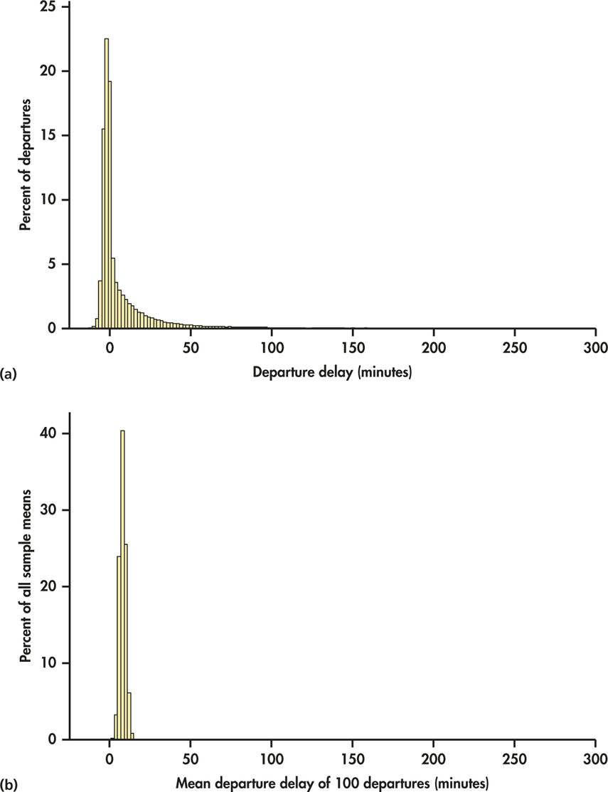
Suppose we take an SRS of 100 fights. The mean delay time in this sample is minutes. That’s less than the mean of the population. Take another SRS of size 100. The mean for this sample is minutes. That’s higher than the mean of the population. If we take more samples of size 100, we will get different values of . To find the sampling distribution of , we take many random samples of size 100 and calculate for each sample. Figure 6.1(b) is a histogram of the mean departure delay times for 1000 samples, each of size 100. The scales and choice of classes are exactly the same as in Figure 6.1(a) so that we can make a direct comparison. Notice something remarkable. Even though the distribution of the individual delay times is strongly skewed and very spread out, the distribution of the sample means is quite symmetric and much less spread out.
291
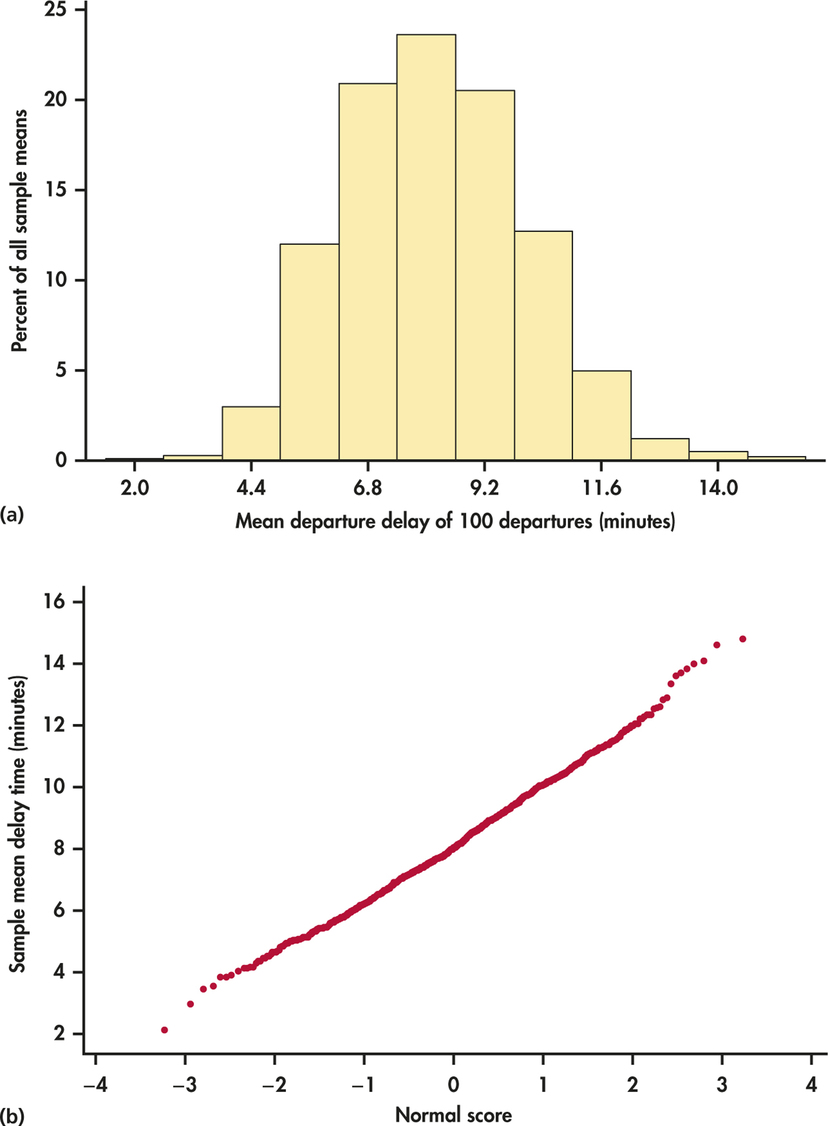
Figure 6.2(a) is the histogram of the sample means on a scale that more clearly shows its shape. We can see that the distribution of sample means is close to the Normal distribution. The Normal quantile plot of Figure 6.2(b) further confirms the compatibility of the distribution of sample means with the Normal distribution. Furthermore, the histogram in Figure 6.2(a) appears to be essentially centered on the population mean value. Specifically, the mean of the 1000 sample means is 8.01, which is nearly equal to the -value of 7.92.
292
This example illustrates three important points discussed in this section.
Facts about Sample Means
- Sample means are less variable than individual observations.
- Sample means are centered around the population mean.
- Sample means are more Normal than individual observations.
These three facts contribute to the popularity of sample means in statistical inference of the population mean.
The mean and standard deviation of
The sample mean from a sample or an experiment is an estimate of the mean of the underlying population. The sampling distribution of is determined by the design used to produce the data, the sample size , and the population distribution.
Select an SRS of size from a population, and measure a variable on each individual case in the sample. The measurements are values of random variables . A single is a measurement on one individual case selected at random from the population and, therefore, has the distribution of the population. If the population is large relative to the sample, we can consider to be independent random variables each having the same distribution. This is our probability model for measurements on each individual case in an SRS.
The sample mean of an SRS of size is
If the population has mean , then is the mean of the distribution of each observation . To get the mean of we use the rules for means of random variables. Specifically,
Reminder
rules for means, p. 226
Reminder
rules for variances, p. 231
That is, the mean of is the same as the mean of the population. The sample mean is therefore an unbiased estimator of the unknown population mean .
The observations are independent, so the addition rule for variances also applies:
With in the denominator, the variability of about its mean decreases as the sample size grows. Thus, a sample mean from a large sample will usually be very close to the true population mean . Here is a summary of these facts.
293
Mean and Standard Deviation of a Sample Mean
Let be the mean of an SRS of size from a population having mean and standard deviation. The mean and standard deviation of are
Reminder
unbiased estimator, p. 279
How precisely does a sample mean estimate a population mean ? Because the values of vary from sample to sample, we must give an answer in terms of the sampling distribution. We know that is an unbiased estimator of , so its values in repeated samples are not systematically too high or too low. Most samples will give an -value close to if the sampling distribution is concentrated close to its mean . So the precision of estimation depends on the spread of the sampling distribution.
Because the standard deviation of is the standard deviation of the statistic decreases in proportion to the square root of the sample size. This means, for example, that a sample size must be multiplied by 4 in order to divide the statistic’s standard deviation in half. By comparison, a sample size must be multiplied by 100 in order to reduce the standard deviation by a factor of 10.
EXAMPLE 6.3 Standard Deviations for Sample Means of Departure Delays
The standard deviation of the population of departure delays in Figure 6.1(a) is minutes. The delay of any single departure will often be far from the population mean. If we choose an SRS of 25 departures, the standard deviation of their mean length is
Averaging over more departures reduces the variability and makes it more likely that is close to . Our sample size of 100 departures is , so the standard deviation will be half as large:
Apply Your Knowledge
Question 6.2
6.2 Find the mean and the standard deviation of the sampling distribution.
Compute the mean and standard deviation of the sampling distribution of the sample mean when you plan to take an SRS of size 49 from a population with mean 420 and standard deviation 21.
Question 6.3
6.3 The effect of increasing the sample size.
In the setting of the previous exercise, repeat the calculations for a sample size of 441. Explain the effect of the sample size increase on the mean and standard deviation of the sampling distribution.
6.3
. Larger sample gives the same mean but a smaller standard deviation.
294
The central limit theorem
We have described the center and spread of the probability distribution of a sample mean , but not its shape. The shape of the distribution of depends on the shape of the population distribution. Here is one important case: if the population distribution is Normal, then so is the distribution of the sample mean.
Sampling Distribution of a Sample Mean
If a population has the . distribution, then the sample mean of independent observations has the distribution.
This is a somewhat special result. Many population distributions are not exactly Normal. The delay departures in Figure 6.1(a), for example, are extremely skewed. Yet Figures 6.1(b) and 6.2 show that means of samples of size 100 are close to Normal. One of the most famous facts of probability theory says that, for large sample sizes, the distribution of is close to a Normal distribution. This is true no matter what shape the population distribution has, as long as the population has a finite standard deviation . This is the central limit theorem. It is much more useful than the fact that the distribution of is exactly Normal if the population is exactly Normal.
Central Limit Theorem
Draw an SRS of size from any population with mean and finite standard deviation . When is large, the sampling distribution of the sample mean is approximately Normal:
EXAMPLE 6.4 How Close will the Sample Mean Be to the Population Mean?
With the Normal distribution to work with, we can better describe how precisely a random sample of 100 departures estimates the mean departure delay of all the departures in the population. The population standard deviation for the more than 210,000 departures in the population of Figure 6.1(a) is minutes. From Example 6.3, we know minutes. By the 95 part of the 68–95–99.7 rule, about 95% of all samples will have its mean within two standard deviations of , that is, within ±5.16 of .
Reminder
68-95-99.7 rule, p. 43
Apply Your Knowledge
Question 6.4
6.4 Use the 68–95–99.7 rule.
You take an SRS of size 49 from a population with mean 185 and standard deviation 70. According to the central limit theorem, what is the approximate sampling distribution of the sample mean? Use the 95 part of the 68–95–99.7 rule to describe the variability of .
The population of departure delays is very spread out, so the sampling distribution of has a large standard deviation. If we view the sample mean based on as not sufficiently precise, then we must consider an even larger sample size.
295
EXAMPLE 6.5 How Can we Reduce the Standard Deviation of the Sample Mean?
In the setting of Example 6.4, if we want to reduce the standard deviation of by a factor of 4, we must take a sample 16 times as large, , or 1600. Then
For samples of size 1600, about 95% of the sample means will be within twice 0.65, or 1.3 minutes, of the population mean .
Apply Your Knowledge
Question 6.5
6.5 The effect of increasing the sample size.
In the setting of Exercise 6.4, suppose that we increase the sample size to 1225. Use the 95 part of the 68–95–99.7 rule to describe the variability of this sample mean. Compare your results with those you found in Exercise 6.4.
6.5
.
Example 6.5 reminds us that if the population is very spread out, the in the standard deviation of implies that very large samples are needed to estimate the population mean precisely. The main point of the example, however, is that the central limit theorem allows us to use Normal probability calculations to answer questions about sample means even when the population distribution is not Normal.
How large a sample size is needed for to be close to Normal depends on the population distribution. More observations are required if the shape of the population distribution is far from Normal. For the very skewed departure delay population, samples of size 100 are large enough. Further study would be needed to see if the distribution of is close to Normal for smaller samples like or . Here is a more detailed study of another skewed distribution.
EXAMPLE 6.6 The Central Limit Theorem in Action
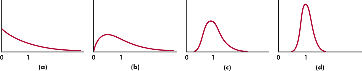
Figure 6.3 shows the central limit theorem in action for another very non-Normal population. Figure 6.3(a) displays the density curve of a single observation from the population. The distribution is strongly right-skewed, and the most probable outcomes are near 0. The mean of this distribution is 1, and its standard deviation is also 1. This particular continuous distribution is called an exponential distribution. Exponential distributions are used as models for how long an iOS device, for example, will last and for the time between text messages sent on your cell phone.
exponential distribution
296
Figures 6.3(b), (c), and (d) are the density curves of the sample means of 2, 10, and 25 observations from this population. As increases, the shape becomes more Normal. The mean remains at , but the standard deviation decreases, taking the value The density curve for 10 observations is still somewhat skewed to the right but already resembles a Normal curve having and . The density curve for is yet more Normal. The contrast between the shape of the population distribution and of the distribution of the mean of 10 or 25 observations is striking.

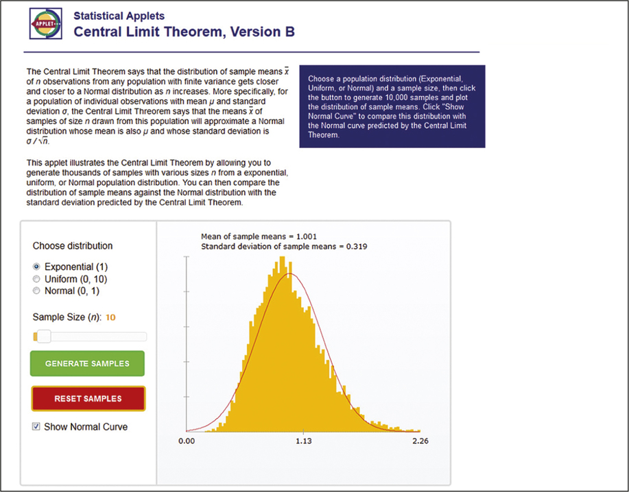
You can also use the Central Limit Theorem applet to study the sampling distribution of . From one of three population distributions, 10,000 SRSs of a user-specified sample size are generated, and a histogram of the sample means is constructed. You can then compare this estimated sampling distribution with the Normal curve that is based on the central limit theorem.
EXAMPLE 6.7 Using the Central Limit Theorem Applet
In Example 6.6, we considered sample sizes of from an exponential distribution. Figure 6.4 shows a screenshot of the Central Limit Theorem applet for the exponential distribution when . The mean and standard deviation of this sampling distribution are 1 and , respectively. From the 10,000 SRSs, the mean is estimated to be 1.001, and the estimated standard deviation is 0.319. These are both quite close to the true values. In Figure 6.3(c), we saw that the density curve for 10 observations is still somewhat skewed to the right. We can see this same behavior in Figure 6.4 when we compare the histogram with the Normal curve based on the central limit theorem.
297
Try using the applet for the other sample sizes in Example 6.6. You should get histograms shaped like the density curves shown in Figure 6.3. You can also consider other sample sizes by sliding from 1 to 100. As you increase , the shape of the histogram moves closer to the Normal curve that is based on the central limit theorem.
Apply Your Knowledge
Question 6.6
6.6 Use the Central Limit Theorem applet.
Let’s consider the uniform distribution between 0 and 10. For this distribution, all intervals of the same length between 0 and 10 are equally likely. This distribution has a mean of 5 and standard deviation of 2.89.
- Approximate the population distribution by setting and clicking the “Generate samples” button.
- What are your estimates of the population mean and population standard deviation based on the 10,000 SRSs? Are these population estimates close to the true values?
- Describe the shape of the histogram and compare it with the Normal curve.
Question 6.7
6.7 Use the Central Limit Theorem applet again.
Refer to the previous exercise. In the setting of Example 6.6, let’s approximate the sampling distribution for samples of size observations.
- For each sample size, compute the mean and standard deviation of
- For each sample size, use the applet to approximate the sampling distribution. Report the estimated mean and standard deviation. Are they close to the true values calculated in part (a)?
- For each sample size, compare the shape of the sampling distribution with the Normal curve based on the central limit theorem.
- For this population distribution, what sample size do you think is needed to make you feel comfortable using the central limit theorem to approximate the sampling distribution of ? Explain your answer.
Now that we know that the sampling distribution of the sample mean is approximately Normal for a sufficiently large , let’s consider some probability calculations.
EXAMPLE 6.8 Time between Sent Text Messages
In Example 5.19 (page 270), it was reported that Americans aged 18 to 29 years send an average of almost 88 text messages a day. Suppose that the time between text messages sent from your cell phone is governed by the exponential distribution with mean minutes and standard deviation minutes. You record the next 50 times between sent text messages. What is the probability that their average exceeds 13 minutes?
The central limit theorem says that the sample mean time (in minutes) between text messages has approximately the Normal distribution with mean equal to the population mean minutes and standard deviation
The sampling distribution of is, therefore, approximately . Figure 6.5 shows this Normal curve (solid) and also the actual density curve of (dashed).
298
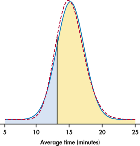
The probability we want is . This is the area to the right of 13 under the solid Normal curve in Figure 6.5. A Normal distribution calculation gives
The exactly correct probability is the area under the dashed density curve in the figure. It is 0.8271. The central limit theorem Normal approximation is off by only about 0.0007.
Apply Your Knowledge
Question 6.8
6.8 Find a probability.
Refer to Example 6.8. Find the probability that the mean time between text messages is less than 16 minutes. The exact probability is 0.6944. Compare your answer with the exact one.
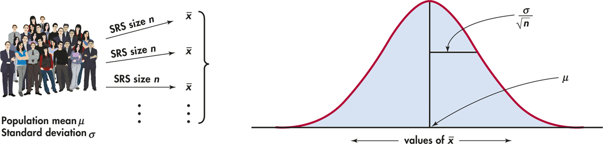
Figure 6.6 summarizes the facts about the sampling distribution of in a way that emphasizes the big idea of a sampling distribution. The general framework for constructing the sampling distribution of is shown on the left.
- Take many random samples of size from a population with mean and standard deviation .
- Find the sample mean for each sample.
- Collect all the ’s and display their distribution.
The sampling distribution of is shown on the right. Keep this figure in mind as you go forward.
The central limit theorem is one of the most remarkable results in probability theory. Our focus was on its effect on averages of random samples taken from any single population. But it is worthwhile to point out two more facts. First, more general versions of the central limit theorem say that the distribution of a sum or average of many small random quantities is close to Normal. This is true even if the quantities are not independent (as long as they are not too highly correlated) and even if they have different distributions (as long as no single random quantity is so large that it dominates the others). These more general versions of the central limit theorem suggest why the Normal distributions are common models for observed data. Any variable that is a sum of many small random influences will have approximately a Normal distribution.
299
Reminder
binomial random variable as a sum, p. 254
The second fact is that the central limit theorem also applies to discrete random variables. An average of discrete random variables will never result in a continuous sampling distribution, but the Normal distribution often serves as a good approximation. Indeed, the central limit theorem tells us why counts and proportions of Chapter 5 are well approximated by the Normal distribution. For the binomial situation, recall that we can consider the count as a sum
of independent random variables that take the value 1 if a success occurs on the th trial and the value 0 otherwise. The proportion of successes can then be thought of as the sample mean of the . And, as we have just learned, the central limit theorem says that sums and averages are approximately Normal when is large. These are indeed the Normal approximation facts for sample counts and proportions we learned and applied in Chapter 5.