6.3 Tests of Significance
The confidence interval is appropriate when our goal is to estimate population parameters. The second common type of inference is directed at a quite different goal: to assess the evidence provided by the data in favor of some claim about the population parameters.
The reasoning of significance tests
A significance test is a formal procedure for comparing observed data with a hypothesis whose truth we want to assess. The hypothesis is a statement about the parameters in a population or model. The results of a test are expressed in terms of a probability that measures how well the data and the hypothesis agree. We use the following Case Study and subsequent examples to illustrate these ideas.
317
CASE 6.1 Fill the Bottles

Perhaps one of the most common applications of hypothesis testing of the mean is the quality control problem of assessing whether or not the underlying population mean is on “target.” Consider the case of Bestea Bottlers. One of Bestea’s most popular products is the 16-ounce or 473-milliliter (ml) bottle of sweetened green iced tea. Annual production at any of its given facilities is in the millions of bottles. There is some variation from bottle to bottle because the filling machinery is not perfectly precise. Bestea has two concerns: whether there is a problem of underfilling (customers are then being shortchanged, which is a form of false advertising) or whether there is a problem of overfilling (unnecessary cost to the bottler).
Notice that in Case 6.1, there is an intimate understanding of what is important to be discovered. In particular, is the population mean too high or too low relative to a desired level? With an understanding of what role the data play in the discovery process, we are able to formulate appropriate hypotheses. If the bottler were concerned only about the possible underfilling of bottles, then the hypotheses of interest would change. Let us proceed with the question of whether the bottling process is either underfilling or overfilling bottles.
EXAMPLE 6.13 Are the Bottles Being Filled as Advertised?
bestea1
CASE 6.1 The filling process is not new to Bestea. Data on past production shows that the distribution of the contents is close to Normal, with standard deviation . To assess the state of the bottling process, 20 bottles were randomly selected from the streaming high volume production line. The sample mean content () is found to be 474.54 ml. Is a sample mean of 474.54 ml convincing evidence that the mean fill of all bottles produced by the current process differs from the desired level of 473 ml?
If we lack proper statistical thinking, this is a juncture to knee-jerk one of two possible conclusions:
- Conclude that “The mean of the bottles sampled is not 473 ml so the process is not filling the bottles at a mean level of 473 ml.”
- Conclude that “The difference of 1.54 ml is small relative to the 473 ml baseline so there is nothing unusual going on here.”
Both responses fail to consider the underlying variability of the population, which ultimately implies a failure to consider the sampling variability of the mean statistic.
So, what is the conclusion? One way to answer this question is to compute the probability of observing a sample mean at least as far from 473 ml as 1.54 ml, assuming, in fact, the underlying process mean is equal to 473 ml. Taking into account sampling variability, the answer is 0.00058. (You learn how to find this probability in Example 6.18.) Because this probability is so small, we see that the sample mean is incompatible with a population mean of . With this evidence, we are led to the conclusion that the underlying bottling process does not have mean of . The estimated average overfilling amount of 1.54 ml per bottle may seem fairly inconsequential. But, when it is put in the context of the high-volume production bottling environment and the potential cumulative waste across many bottles, then correcting the potential overfilling is of great practical importance.
318
What are the key steps in this example?
- We started with a question about the underlying mean of the current filling process. We then ask whether or not the data from process are compatible with a mean fill of 473 ml.
- Next we compared the mean given by the data, , with the value assumed in the question, 473 ml.
- The result of the comparison takes the form of a probability, 0.00058.
The probability is quite small. Something that happens with probability 0.00058 occurs only about six times out of 10,000. In this case, we have two possible explanations:
- We have observed something that is very unusual.
- The assumption that underlies the calculation (underlying process mean equals 473 ml) is not true.
Because this probability is so small, we prefer the second conclusion: the process mean is not 473 ml. It should be emphasized that to “conclude” does not mean we know the truth or that we are right. There is always a chance that our conclusion is wrong. Always bear in mind that when dealing with data, there are no guarantees. We now turn to an example in which the data suggest a different conclusion.
EXAMPLE 6.14 Is It Right now?
bestea2
CASE 6.1 In Example 6.13, sample evidence suggested that the mean fill amount was not at the desired target of 473 ml. In particular, it appeared that the process was overfilling the bottles on average. In response, Bestea’s production staff made adjustments to the process and collected a sample of 20 bottles from the “corrected” process. From this sample, we find . (We assume that the standard deviation is the same, .) In this case, the sample mean is less than 473 ml—to be exact, 0.44 ml less than 473 ml.
Did the production staff overreact and adjust the mean level too low? We need to ask a similar question as in Example 6.13. In particular, what is the probability that the mean of a sample of size from a Normal population with mean and standard deviation is as far away or farther away from 473 ml as 0.44 ml? The answer is 0.328. A sample result this far from 473 ml would happen just by chance in 32.8% of samples from a population having a true mean of 473 ml. An outcome that could so easily happen just by chance is not convincing evidence that the population mean differs from 473 ml.
At this moment, Bestea does not have strong evidence to further tamper with the process settings. But, with this said, no decision is static or necessarily correct. Considering the cost of underfilling in terms of disgruntled customers is potentially greater than the waste cost of overfilling, Bestea personnel might be well served to gather more data if there is any suspicion that the process mean fill amount is too low. In Section 6.5, we discuss sample size considerations for detecting departures from the null hypothesis that are considered important given a specified probability of detection.
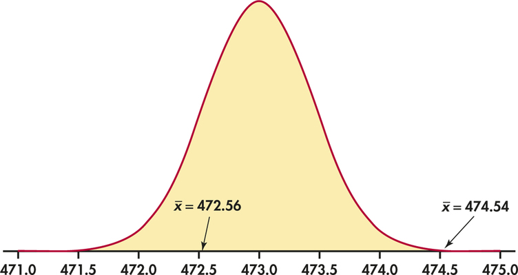
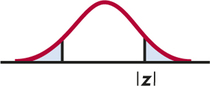
The probabilities in Examples 6.13 and 6.14 are measures the compatibility of the data (sample means of 474.54 and 472.56) with the null hypothesis that . Figure 6.12 compares these two results graphically. The Normal curve is the sampling distribution of when . You can see that we are not particularly surprised to observe , but is clearly an unusual data result. Herein lies the core reasoning of statistical tests: a data result that is extreme if a hypothesis were true is evidence that the hypothesis may not be true. We now consider some of the formal aspects of significance testing.
319
Stating hypotheses
In Examples 6.13 and 6.14, we asked whether the fill data are plausible if, in fact, the true mean fill amount for all bottles ( ) is 473 ml. That is, we ask if the data provide evidence against the claim that the population mean is 473. The first step in a test of significance is to state a claim that we will try to find evidence against.
Null Hypothesis
The statement being tested in a test of significance is called the null hypothesis. The test of significance is designed to assess the strength of the evidence against the null hypothesis. Usually, the null hypothesis is a statement of “no effect” or “no difference.” We abbreviate “null hypothesis” as .
A null hypothesis is a statement about the population or process parameters. For example, the null hypothesis for Examples 6.13 and 6.14 is
Note that the null hypothesis refers to the process mean for all filled bottles, including those we do not have data on.
alternative hypothesis
It is convenient also to give a name to the statement that we hope or suspect is true instead of . This is called the alternative hypothesis and is abbreviated as . In Examples 6.13 and 6.14, the alternative hypothesis states that the mean fill amount is not 473. We write this as

Hypotheses always refer to some population, process, or model, not to a particular data outcome. For this reason, we always state and in terms of population parameters.
Because expresses the effect that we hope to find evidence for, we will sometimes begin with and then set up as the statement that the hoped-for effect is not present. Stating , however, is often the more diffcult task. It is not always clear, in particular, whether should be one-sided or two-sided, which refers to whether a parameter differs from its null hypothesis value in a specific direction or in either direction.
one-sided or two-sided alternatives
320
The alternative in the bottle-filling examples is two-sided. In both examples, we simply asked if mean fill amount is off target. The process can be off target in that it fills too much or too little on average, so we include both possibilities in the alternative hypothesis. Here, the alternative is not a good situation in the sense that the process mean is off target. Thus, it is not our hope the alternative is true. It, however, is our hope that we can detect when the process has gone off target so that corrective actions can be done. Here is a setting in which a one-sided alternative is appropriate.
EXAMPLE 6.15 Have We Reduced Processing Time?
Your company hopes to reduce the mean time required to process customer orders. At present, this mean is 3.8 days. You study the process and eliminate some unnecessary steps. Did you succeed in decreasing the average processing time? You hope to show that the mean is now less than 3.8 days, so the alternative hypothesis is one-sided, . The null hypothesis is as usual the “no-change” value, days.
The alternative hypothesis should express the hopes or suspicions we bring to the data. It is cheating to first look at the data and then frame to fit what the data show. If you do not have a specific direction firmly in mind in advance, you must use a two-sided alternative. Moreover, some users of statistics argue that we should always use a two-sided alternative.
The choice of the hypotheses in Example 6.15 as
deserves a final comment. We do not expect that elimination of steps in order processing would actually increase the processing time. However, we can allow for an increase by including this case in the null hypothesis. Then we would write
This statement is logically satisfying because the hypotheses account for all possible values of . However, only the parameter value in that is closest to influences the form of the test in all common significance-testing situations. Think of it this way: if the data lead us away from to believing that , then the data would certainly lead us away from believing that because this involves values of that are in the opposite direction to which the data are pointing. Moving forward, we take to be the simpler statement that the parameter equals a specific value, in this case .
Apply Your Knowledge
Question 6.51
6.51 Customer feedback.
Feedback from your customers shows that many think it takes too long to fill out the online order form for your products. You redesign the form and plan a survey of customers to determine whether or not they think that the new form is actually an improvement. Sampled customers will respond using a 5-point scale: if the new form takes much less time than the old form; if the new form takes a little less time; 0 if the new form takes about the same time; if the new form takes a little more time; and if the new form takes much more time. The mean response from the sample is , and the mean response for all of your customers is State null and alternative hypotheses that provide a framework for examining whether or not the new form is an improvement.
321
6.51
.
Question 6.52
6.52 Laboratory quality control.
Hospital laboratories routinely check their diagnostic equipment to ensure that patient lab test results are accurate. To check if the equipment is well calibrated, lab technicians make several measurements on a control substance known to have a certain quantity of the chemistry being measured. Suppose a vial of controlled material has 4.1 nanomoles per L of potassium. The technician runs the lab equipment on the control material 10 times and compares the sample mean reading with the theoretical mean using a significance test. State the null and alternative hypotheses for this test.
Test statistics
We learn the form of significance tests in a number of common situations. Here are some principles that apply to most tests and that help in understanding the form of tests:
- The test is based on a statistic that estimates the parameter that appears in the hypotheses. Usually, this is the same estimate we would use in a confidence interval for the parameter. When is true, we expect the estimate to take a value near the parameter value specified by . We call this specified value the hypothesized value.
- Values of the estimate far from the hypothesized value give evidence against . The alternative hypothesis determines which directions count against .
- To assess how far the estimate is from the hypothesized value, standardize the estimate. In many common situations, the test statistic has the form
test statistic
A test statistic measures compatibility between the null hypothesis and the data. We use it for the probability calculation that we need for our test of significance. It is a random variable with a distribution that we know.
Let’s return to our bottle filling example and specify the hypotheses as well as calculate the test test statistic.
EXAMPLE 6.16 Bottle Fill Amount: The Hypotheses
CASE 6.1 For Examples 6.13 and 6.14 (pages 317 and 318), the hypotheses are stated in terms of the mean fill amount for all bottles:
The estimate of is the sample mean . Because is two-sided, values of far from 473 on either the low or the high side count as evidence against the null hypothesis.
322
EXAMPLE 6.17 Bottle Fill Amount: The Test Statistic
CASE 6.1 For Example 6.13 (page 317), the null hypothesis is , and a sample gave . The test statistic for this problem is the standardized version of :
This statistic is the distance between the sample mean and the hypothesized population mean in the standard scale of -scores. In this example,
Reminder

68-95-99.7 rule, p. 43
Even without a formal probability calculation, by simply recalling the 68–95–99.7 rule for the Normal, we realize that a -score of 3.44 is an unusual value. This suggests incompatibility of the observed sample result with the null hypothesis.
As stated in Example 6.13, past production shows that the fill amounts of the individual bottles are not too far from the Normal distribution. In that light, we can be confident enough that, with a sample size of 20, the distribution of the sample is close enough to the Normal for working purposes. In turn, the standardized test statistic will have approximately the distribution. We use facts about the Normal distribution in what follows.
-values
If all test statistics were Normal, we could base our conclusions on the value of the test statistic. In fact, the Supreme Court of the United States has said that “two or three standard deviations” ( is its criterion for rejecting (see Exercise 6.59, page 326), and this is the criterion used in most applications involving the law. But because not all test statistics are Normal, as we learn in subsequent chapters, we use the language of probability to express the meaning of a test statistic.
A test of significance finds the probability of getting an outcome as extreme or more extreme than the actually observed outcome. “Extreme” means “far from what we would expect if were true.” The direction or directions that count as “far from what we would expect” are determined by and .
-Value
The probability, computed assuming that is true, that the test statistic would take a value as extreme or more extreme than that actually observed is called the -value of the test. The smaller the -value, the stronger the evidence against provided by the data.
The key to calculating the -value is the sampling distribution of the test statistic. For the problems we consider in this chapter, we need only the standard Normal distribution for the test statistic .
EXAMPLE 6.18 Bottle Fill Amount: The -Value
CASE 6.1 In Example 6.13, the observations are an SRS of size from a population of bottles with . The observed average fill amount is . In Example 6.17, we found that the test statistic for testing versus is
323
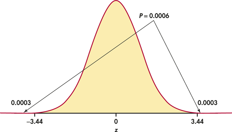
If is true, then is a single observation from the standard Normal, (0,1), distribution. Figure 6.13 illustrates this calculation. The -value is the probability of observing a value of at least as extreme as the one that we observed, . From Table A, our table of standard Normal probabilities, we find
The probability for being extreme in the negative direction is the same:
So the -value is
In Example 6.13 (page 317), we reported a probability of 0.00058 was obtained from software. The value of 0.0006 found from the tables is essentially the same.
Apply Your Knowledge
Question 6.53
6.53 Spending on housing.
The Census Bureau reports that households spend an average of 31% of their total spending on housing. A homebuilders association in Cleveland wonders if the national finding applies in its area. It interviews a sample of 40 households in the Cleveland metropolitan area to learn what percent of their spending goes toward housing. Take to be the mean percent of spending devoted to housing among all Cleveland households. We want to test the hypotheses
The population standard deviation is .
- The study finds for the 40 households in the sample. What is the value of the test statistic ? Sketch a standard Normal curve, and mark on the axis. Shade the area under the curve that represents the -value.
- Calculate the -value. Are you convinced that Cleveland differs from the national average?
324
6.53
(a) . (b) 0.1142. No.
Question 6.54
6.54 State null and alternative hypotheses.
In the setting of the previous exercise, suppose that the Cleveland homebuilders were convinced, before interviewing their sample, that residents of Cleveland spend less than the national average on housing. Do the interviews support their conviction? State null and alternative hypotheses. Find the -value, using the interview results given in the previous problem. Why do the same data give different -values in these two problems?
Question 6.55
6.55 Why is this wrong?
The homebuilders wonder if the national finding applies in the Cleveland area. They have no idea whether Cleveland residents spend more or less than the national average. Because their interviews find that , less than the national 31%, their analyst tests
Explain why this is incorrect.
6.55
You shouldn’t look at the data before deciding the hypotheses; they should be determined based on prior knowledge beforehand.
Statistical significance
We started our discussion of significance tests with the statement of null and alternative hypotheses. We then learned that a test statistic is the tool used to examine the compatibility of the observed data with the null hypothesis. Finally, we translated the test statistic into a -value to quantify the evidence against . One important final step is needed: to state our conclusion.
significance level
We can compare the -value we calculated with a fixed value that we regard as decisive. This amounts to announcing in advance how much evidence against we will require to reject . The decisive value is called the significance level. It is commonly denoted by (the Greek letter alpha). If we choose , we are requiring that the data give evidence against so strong that it would happen no more than 5% of the time (1 time in 20) when is true. If we choose , we are insisting on stronger evidence against , evidence so strong that it would appear only 1% of the time (1 time in 100) if is, in fact, true.
Statistical Significance
If the -value is as small or smaller than , we say that the data are statistically signifcant at level .
“Signifcant” in the statistical sense does not mean “important.” The original meaning of the word is “signifying something.” In statistics, the term is used to indicate only that the evidence against the null hypothesis has reached the standard set by . For example, significance at level 0.01 is often expressed by the statement “The results were signifcant .” Here stands for the -value. The -value is more informative than a statement of significance because we can then assess significance at any level we choose. For example, a result with is signifcant at the level but is not signifcant at the level. We discuss this in more detail at the end of this section.
EXAMPLE 6.19 Bottle Fill Amount: The Conclusion
CASE 6.1 In Example 6.18, we found that the -value is
325
If the underlying process mean is truly 473 ml, there is only a 6 in a 10,000 chance of observing a sample mean deviating as extreme as 1.54 ml (in either direction) away from this hypothesized mean. Because this -value is smaller than the significance level, we conclude that our test result is signifcant. We could report the result as “the data clearly show evidence that the underlying process mean filling amount is not at the desired value of 473 ml (, ).”
Note that the calculated -value for this example is actually 0.0006, but we reported the result as . The value 0.001, 1 in 1000, is sufficiently small to force a clear rejection of . When encountering a very small -value as in Example 6.19, standard practice is to provide the test statistic value and report the -value as simply less than 0.001.
Examples 6.16 through 6.19 in sequence showed us that a test of significance is a process for assessing the significance of the evidence provided by the data against a null hypothesis. These steps provide the general template for all tests of significance. Here is a general summary of the four common steps.
Test of Significance: Common Steps
- State the null hypothesis and the alternative hypothesis . The test is designed to assess the strength of the evidence against ; is the statement that we accept if the evidence enables us to reject .
- Calculate the value of the test statistic on which the test will be based. This statistic usually measures how far the data are from .
- Find the P-value for the observed data. This is the probability, calculated assuming that is true, that the test statistic will weigh against at least as strongly as it does for these data.
- State a conclusion. One way to do this is to choose a significance level , how much evidence against you regard as decisive. If the -value is less than or equal to, you conclude that the alternative hypothesis is true; if it is greater than , you conclude that the data do not provide sufficient evidence to reject the null hypothesis. Your conclusion is a sentence or two that summarizes what you have found by using a test of significance.
We learn the details of many tests of significance in the following chapters. The proper test statistic is determined by the hypotheses and the data collection design. We use computer software or a calculator to find its numerical value and the -value. The computer will not formulate your hypotheses for you, however. Nor will it decide if significance testing is appropriate or help you to interpret the -value that it presents to you. These steps require judgment based on a sound understanding of this type of inference.
Apply Your Knowledge
Question 6.56
6.56 Finding signifcant -scores.
Consider a two-sided significance test for a population mean.
- Sketch a Normal curve similar to that shown in Figure 6.13 (page 323), but find the value such that .
- Based on your curve from part (a), what values of the statistic are statistically signifcant at the level?
326
Question 6.57
6.57 Significance.
You are testing against based on an SRS of 30 observations from a Normal population. What values of the statistic are statistically signifcant at the level?
6.57
.
Question 6.58
6.58 Significance.
You are testing against based on an SRS of 30 observations from a Normal population. What values of the statistic are statistically signifcant at the level?
Question 6.59
6.59 The Supreme Court speaks.
Court cases in such areas as employment discrimination often involve statistical evidence. The Supreme Court has said that -scores beyond are generally convincing statistical evidence. For a two-sided test, what significance level corresponds to ? To ?
6.59
0.0456. 0.0026.
Tests of one population mean
We have noted the four steps common to all tests of significance. We have also illustrated these steps with the bottle filling scenario of Case 6.1 (page 317). Here is a summary for the test of one population mean.
We want to test a population parameter against a specified value. This is the null hypothesis. For a test of a population mean , the null hypothesis is
which often is expressed as
where is the hypothesized value of that we would like to examine.
The test is based on data summarized as an estimate of the parameter. For a population mean, this is the sample mean . Our test statistic measures the difference between the sample estimate and the hypothesized parameter in terms of standard deviations of the test statistic:
Recall from Section 6.1 that the standard deviation of is . Therefore, the test statistic is
Again recall from Section 6.1 that, if the population is Normal, then will be Normal and will have the standard Normal distribution when is true. By the central limit theorem, both distributions will be approximately Normal when the sample size is large, even if the population is not Normal. We assume that we’re in one of these two settings for now.
Suppose that we have calculated a test statistic . If the alternative is one-sided on the high side, then the -value is the probability that a standard Normal random variable takes a value as large or larger than the observed 1.7. That is,
Similar reasoning applies when the alternative hypothesis states that the true lies below the hypothesized (one-sided). When states that is simply unequal to (two-sided), values of away from zero in either direction count against the null hypothesis. The -value is the probability that a standard Normal is at least as far from zero as the observed . Again, if the test statistic is , the two-sided -value is the probability that or . Because the standard Normal distribution is symmetric, we calculate this probability by finding and doubling it:
327
We would make exactly the same calculation if we observed . It is the absolute value that matters, not whether is positive or negative. Here is a statement of the test in general terms.
Test for a Population Mean
To test the hypothesis : based on an SRS of size from a population with unknown mean and known standard deviation , compute the test statistic
In terms of a standard Normal random variable , the -value for a test of against
These -values are exact if the population distribution is Normal and are approximately correct for large in other cases.
EXAMPLE 6.20 Blood Pressures of Executives
The medical director of a large company is concerned about the effects of stress on the company’s younger executives. According to the National Center for Health Statistics, the mean systolic blood pressure for males 35 to 44 years of age is 128, and the standard deviation in this population is 15. The medical director examines the records of 72 executives in this age group and finds that their mean systolic blood pressure is . Is this evidence that the mean blood pressure for all the company’s young male executives is higher than the national average? As usual in this chapter, we make the unrealistic assumption that the population standard deviation is known—in this case, that executives have the same as the general population.
Step 1: Hypotheses. The hypotheses about the unknown mean of the executive population are
328
Step 2: Test statistic. The test requires that the 72 executives in the sample are an SRS from the population of the company’s young male executives. We must ask how the data were produced. If records are available only for executives with recent medical problems, for example, the data are of little value for our purpose. It turns out that all executives are given a free annual medical exam and that the medical director selected 72 exam results at random. The one-sample statistic is
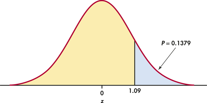
Step 3: P-value. Draw a picture to help find the -value. Figure 6.14 shows that the -value is the probability that a standard Normal variable takes a value of 1.09 or greater. From Table A we find that this probability is
Step 4: Conclusion. We could report the result as “the data fail to provide evidence that would lead us to conclude that the mean blood pressure for company’s young male executives is higher than the general population of men of the same age group (, ).”
The reported statement does not imply that we conclude that the null hypothesis is true, only that the level of evidence we require to reject the null hypothesis is not met. Our criminal court system follows a similar procedure in which a defendant is presumed innocent until proven guilty. If the level of evidence presented is not strong enough for the jury to find the defendant guilty beyond a reasonable doubt, the defendant is acquitted. Acquittal does not imply innocence, only that the degree of evidence was not strong enough to prove guilt.
Apply Your Knowledge
Question 6.60
6.60 Testing a random number generator.
Statistical software has a “random number generator” that is supposed to produce numbers uniformly distributed between 0 and 1. If this is true, the numbers generated come from a population with . A command to generate 100 random numbers gives outcomes with mean and . Because the sample is reasonably large, take the population standard deviation also to be . Do we have evidence that the mean of all numbers produced by this software is not 0.5?
329
Question 6.61
6.61 Computing the test statistic and -value.
You will perform a significance test of based on an SRS of . Assume that .
- If , what is the test statistic ?
- What is the -value if ?
- What is the -value if ?
6.61
(a) . (b) 0.0618. (c) 0.1236.
Question 6.62
6.62 A new supplier.
A new supplier offers a good price on a catalyst used in your production process. You compare the purity of this catalyst with that from your current supplier. The -value for a test of “no difference” is 0.31. Can you be confident that the purity of the new product is the same as the purity of the product that you have been using? Discuss.
Two-sided significance tests and confidence intervals
Recall the basic idea of a confidence interval, discussed in Section 6.2. We constructed an interval that would include the true value of with a specified probability . Suppose that we use a 95% confidence interval . Then the values of that are not in our interval would seem to be incompatible with the data. This sounds like a significance test with (or 5%) as our standard for drawing a conclusion. The following example demonstrates that this is correct.
EXAMPLE 6.21 IPO Initial Returns
The decision to go public is clearly one of the most signifcant decisions to be made by a privately owned company. Such a decision is typically driven by the company’s desire to raise capital and expand its operations. The first sale of stock to the public by a private company is referred to as an initial public offering (IPO). One of the important measurables for the IPO is the initial return which is defined as:
The first-day closing price represents what market investors are willing to pay for the company’s shares. If the offer price is lower than the first-day closing price, the IPO is said to be underpriced and money is “left on the table” for the IPO buyers. In light of the fact that existing shareholders ended up having to settle for a lower price than they offered, the money left on the table represents wealth transfer from existing shareholders to the IPO buyers. In terms of the IPO initial return, an under-priced IPO is associated with a positive initial return. Similarly, an overpriced IPO is associated with a negative initial return.
Numerous studies in the finance literature consistently report that IPOs, on average, are underpriced in U.S. and international markets. The underpricing phenomena represents a perplexing puzzle in finance circles because it seems to contradict the assumption of market efficiency. In a study of Chinese markets, researchers gathered data on 948 IPOs and found the mean initial return to be 66.3% and the standard deviation of the returns was found to be 80.6%.16 A question that might be asked is if the Chinese IPO initial returns are showing a mean return different than 0—that is, neither a tendency toward underpricing nor overpricing. This calls for a test of the hypotheses
We carry out the test twice, first with the usual significance test and then with a 99% confidence interval.
330
First, the test. The mean of the sample is . Given the large sample size of , it is fairly safe to use the reported standard deviation of 80.6% as . The test statistic is
Because the alternative is two-sided, the -value is
The largest value of in Table A is 3.49. Even though we cannot determine the exact probability from the table, it is pretty obvious that the -value is much less than 0.001. There is overwhelming evidence that the mean initial return for the Chinese IPO population is not 0.
To compute a 99% confidence interval for the mean IPO initial return, find in Table D the critical value for 99% confidence. It is , the same critical value that marked off signifcant ’s in our test. The confidence interval is
The hypothesized value falls well outside this confidence interval. In other words, it is in the region we are 99% confident is not in. Thus, we can reject
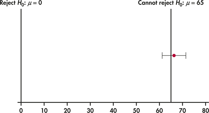
at the 1% significance level. However, we might want to test the Chinese market against other markets. For example, certain IPO markets, such as technology and the “dot-com” markets, have shown abnormally high initial returns. Suppose we wish to test the Chinese market against a market that has value of 65. Because the value of 65 lies inside the 99% confidence interval for , we cannot reject
Figure 6.15 illustrates both cases.
The calculation in Example 6.21 for a 1% significance test is very similar to the calculation for a 99% confidence interval. In fact, a two-sided test at significance level can be carried out directly from a confidence interval with confidence level .
331
Two-Sided Significance Tests and Confidence Intervals
A level two-sided significance test rejects a hypothesis exactly when the value falls outside a level confidence interval for .
Apply Your Knowledge
Question 6.63
6.63 Does the confidence interval include ?
The -value for a two-sided test of the null hypothesis is 0.037.
- Does the 95% confidence interval include the value 20? Explain.
- Does the 99% confidence interval include the value 20? Explain.
6.63
(a) No; because 0.037 is less than 0.05, we reject so that 20 falls outside the 95% confidence interval. (b) Yes; because 0.037 is greater than 0.01, we fail to reject so that 20 is inside the 99% confidence interval.
Question 6.64
6.64 Can you reject the null hypothesis?
A 95% confidence interval for a population mean is (42,51).
- Can you reject the null hypothesis that at the 5% significance level? Why?
- Can you reject the null hypothesis that at the 5% significance level? Why?
-values versus reject-or-not reporting
Imagine that we are conducting a two-sided test and find the observed to be 2.41. Suppose we have picked a significance level of . We can find from Table A or the bottom of Table D, that a value gives us a point on the standard Normal distribution such that 5% of the distribution is beyond ±1.96. Given , we would reject the null hypothesis for . We take the absolute value of the observed because had we gotten a of -2.41, we would need to arrive at the same conclusion of rejection. For one-sided testing with , we would compare our observed with for a less-than alternative and with greater-than alternative.
critical value
A value of that is used to compare the observed against is called a critical value. From our preceding discussion, we could report, “With an observed statistic of 2.41, the data lead us to reject the null hypothesis at the 5% level of significance.” What if the reader of the report sets his or her bar at the 1% level of significance? What would the conclusion of our report be now? The way our report presently stands, we would be forcing the reader to find out for themselves the conclusion at the 1% level. It would be even worse if we did not report the observed value and simply reported that the results are signifcant at the 5% level . It is equally noninformative to report that the results are insignifcant at the 5% level . Clearly, these examples of significance test reporting are very self limiting.
Consider now the reporting of the -value as we have done with all our examples. For the two-sided alternative and an observed of 2.41, the -value is
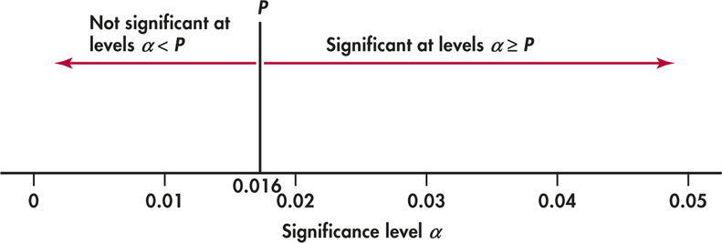
The -value gives a better sense of how strong the evidence is. Notice how much more informative and convenient for others if we report, “The data lead us to reject the null hypothesis (, ).” Namely, we find the result is signifcant at the level because . But, it is not signifcant at the level because the -value is larger than 0.01. From Figure 6.16, we see that the P-value is the smallest level a at which the data are signifcant. With -value in hand, we don’t need to search tables to find different critical values to compare against for different values of . Knowing the -value allows us, or anyone else, to assess sig-nifcance at any level with ease. With this said, the -value is not the “answer all” of a statistical study. As will be emphasized in Section 6.4, a result that is found to be statistically signifcant does not necessarily imply practically important.
332
Our discussion clearly encourages the reporting of -values as opposed to the reject-or-not reporting based on some fixed such as 0.05. The practice of statistics almost always employs computer software or a calculator that calculates -values automatically. In practice, the use of tables of critical values is becoming outdated. Notwithstanding, we include the usual tables of critical values (such as Table D) at the end of the book for learning purposes and to rescue students without computing resources.
Apply Your Knowledge
Question 6.65
6.65 -value and significance level.
The -value for a significance test is 0.023.
- Do you reject the null hypothesis at level ?
- Do you reject the null hypothesis at level ?
- Explain how you determined your answers in parts (a) and (b).
6.65
(a) Yes. (b) No. (c) Because , we reject . Because 0.023 > 0.01, we do not reject .
Question 6.66
6.66 More on -value and significance level.
The -value for a significance test is 0.079.
- Do you reject the null hypothesis at level ?
- Do you reject the null hypothesis at level ?
- Explain how you determined your answers in parts (a) and (b).