7 Inference for Means

7.1 Inference for the Mean of a Population

This page includes Video Technology Manuals

This page includes Statistical Videos

Both confidence intervals and tests of significance for the mean $μ$ of a Normal population are based on the sample mean $\bar{x}$ , which estimates the unknown $μ$ . The sampling distribution of $\bar{x}$ depends on the standard deviation $σ$ . This fact causes no difficulty when $σ$ is known. When $σ$ is unknown, we must estimate $σ$ even though we are primarily interested in $μ$ .

Reminder

sampling distribution of $\bar{x}$ , p. 294

In this section, we meet the sampling distribution of the standardized mean when we use the sample standard deviation $s$ as our estimate of the standard deviation $σ$ . We then use this sampling distribution in our discussion of both confidence intervals and significance tests for inference about the mean $μ$ .

$t$ distributions

Suppose that we have a simple random sample (SRS) of size $n$ from a Normally distributed population with mean $μ$ and standard deviation $σ$ . The sample mean $\bar{x}$ is then Normally distributed with mean $μ$ and standard deviation $σ / \sqrt{n}$ . When $σ$ is not known, we estimate it with the sample standard deviation $s$ , and then we estimate the standard deviation of $\bar{x}$ by $s / \sqrt{n}$ . This quantity is called the standard error of the sample mean $\bar{x}$ , and we denote it by ${SE}_{x}$ .

Standard Error

When the standard deviation of a statistic is estimated from the data, the result is called the standard error of the statistic. The standard error of the sample mean is

${SE}_{\bar{x}} = \frac{s}{\sqrt{n}}$

The term “standard error” is sometimes used for the actual standard deviation of a statistic. The estimated value is then called the “estimated standard error.” In this book, we use the term “standard error” only when the standard deviation of a statistic is estimated from the data. The term has this meaning in the output of many statistical computer packages and in reports of research in many fields that apply statistical methods.

In the previous chapter, the standardized sample mean, or one-sample $z$ statistic,

$z = \frac{\bar{x} - μ}{σ / \sqrt{n}}$

was used to introduce us to the procedures for inference about $μ$ . This statistic has the standard Normal distribution $N (0, 1)$ . However, when we substitute the standard error $s / \sqrt{n}$ for the standard deviation of $\bar{x}$ , this statistic no longer has a Normal distribution. It has a distribution that is new to us, called a $t$ distribution.

Page 359

The $t$ Distributions

Suppose that an SRS of size $n$ is drawn from an $N (μ, σ)$ population. Then the one-sample $t$ statistic

$t = \frac{\bar{x} - μ}{s / \sqrt{n}}$

has the $t$ distribution with $n - 1$ degrees of freedom.

A particular $t$ distribution is specified by its degrees of freedom. We use $t (k)$ to stand for the $t$ distribution with $k$ degrees of freedom. The degrees of freedom for this $t$ statistic come from the sample standard deviation $s$ in the denominator of $t$ . We saw in Chapter 1 that $s$ has $n - 1$ degrees of freedom. Thus, there is a different $t$ distribution for each sample size. There are also other $t$ statistics with different degrees of freedom, some of which we will meet later in this chapter and others we will meet in later chapters.

Reminder

degrees of freedom, p. 31

The $t$ distributions were discovered in 1908 by William S. Gosset. Gosset was a statistician employed by the Guinness brewing company, which prohibited its employees from publishing their discoveries that were brewing related. In this case, the company let him publish under the pen name “Student” using an example that did not involve brewing. The $t$ distributions are often called “Student’s $t$ ” in his honor.

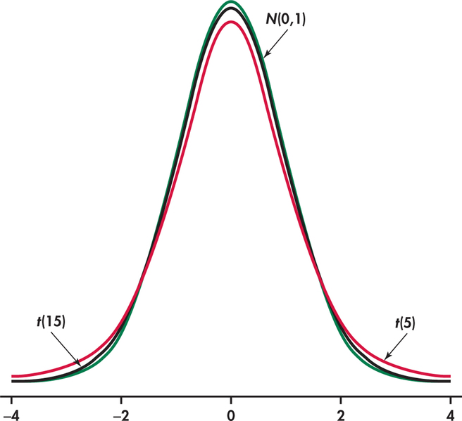
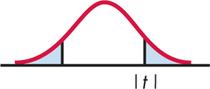
The density curves of the $t (k)$ distributions are similar in shape to the standard Normal curve. That is, they are symmetric about 0 and are bell-shaped. Figure 7.1 compares the density curves of the standard Normal distribution and the $t$ distributions with 5 and 15 degrees of freedom. The similarity in shape is apparent, as is the fact that the $t$ distributions have more probability in the tails and less in the center.

FIGURE 7.1 Density curves for the standard Normal (green),

$t (5)$ (red), and

$t (15)$ (black) distributions. All are symmetric with center 0. The

$t$ distributions have more probability in the tails than the standard Normal distribution.

Page 360

This greater spread is due to the extra variability caused by substituting the random variable $t$ for the fixed parameter $σ$ . Comparing the two $t$ curves, we see that as the degrees of freedom $k$ increase, the $t (k)$ density curve gets closer to the $N (0, 1)$ curve. This reflects the fact that $s$ will generally be closer to $σ$ as the sample size increases.

Apply Your Knowledge

Question 7.1

7.1 One-bedroom rental apartment.

A large city newspaper contains several hundred advertisements for one-bedroom apartments. You choose 25 at random and calculate a mean monthly rent of $703 and a standard deviation of $115.

What is the standard error of the mean?
What are the degrees of freedom for a one-sample $t$ statistic?

7.1

(a) $S E_{\bar{X}} = 23$ . (b) $d f = 24$ .

Question 7.2

7.2 Changing the sample size.

Refer to the previous exercise. Suppose that instead of an SRS of 25, you sampled 16 advertisements.

Would you expect the standard error of the mean to be larger or smaller in this case? Explain your answer.
State why you can’t be certain that the standard error for this new SRS will be larger or smaller.

With the $t$ distributions to help us, we can analyze an SRS from a Normal population with unknown $σ$ or a large sample from a non-Normal population with unknown $σ$ . Table D in the back of the book gives critical values $t^{*}$ for the $t$ distributions. For convenience, we have labeled the table entries both by the value of $p$ needed for significance tests and by the confidence level $C$ (in percent) required for confidence intervals. The standard Normal critical values in the bottom row of entries are labeled $z^{*}$ . This table can be used when you don’t have easy access to computer software.

The one-sample $t$ confidence interval

The one-sample $t$ confidence interval is similar in both reasoning and computational detail to the $z$ procedures of Chapter 6. There, the margin of error for the population mean was $z^{*} σ / \sqrt{n}$ . When $σ$ is unknown, we replace it with its estimate $s$ and switch from $z^{*}$ to $t^{*}$ . This means that the margin of error for the population mean when we use the data to estimate $σ$ is $t^{*} s / \sqrt{n}$ .

Reminder

$z$ confidence interval, p. 307

One-Sample $t$ Confidence Interval

Suppose that an SRS of size $n$ is drawn from a population having unknown mean $μ$ . A level $C$ confidence interval for $μ$ is

$\bar{x} \pm m$

In this formula, the margin of error is

$m = t^{*} {SE}_{\bar{x}} = t^{*} \frac{s}{\sqrt{n}}$

where $t^{*}$ is the value for the $t (n - 1)$ density curve with area $C$ between $- t^{*}$ and $t^{*}$ . This interval is exact when the population distribution is Normal and is approximately correct for large $n$ in other cases.

Page 361

CASE 7.1 Time Spent Using a Smartphone

To mark the launch of a new smartphone, Samsung and $O_{2}$ commissioned a survey of 2000 adult smartphone users in the United Kingdom to better understand how smartphones are being used and integrated into everyday life.¹ Their research found that British smartphone users spend an average of 119 minutes a day on their phones. Making calls was the fifth most time-consuming activity behind browsing the Web (24 minutes), checking social networks (16 minutes), listening to music (15 minutes), and playing games (12 minutes). It appears that students at your institution tend to substitute tablets for many of these activities, thereby possibly reducing the total amount of time they are on their smartphones. To investigate this, you carry out a similar survey at your institution.

EXAMPLE 7.1 Estimating the Average Time Spent on a Smartphone

smrtphn

CASE 7.1 The following data are the daily number of minutes for an SRS of 8 students at your institution:

117

156

116

125

101

100

We want to find a 95% confidence interval for $μ$ , the average number of minutes per day a student uses his or her smartphone.

The sample mean is

$\bar{x} = \frac{117 + 156 + \dots + 100}{8} = 109.5$

and the standard deviation is

$s = \sqrt{\frac{{(117 - 109.5)}^{2} + {(156 - 109.5)}^{2} + \dots + {(100 - 109.5)}^{2}}{8 - 1}} = 25.33$

with degrees of freedom $n - 1 = 7$ . The standard error of $\bar{x}$ is

${SE}_{\bar{x}} = \frac{s}{\sqrt{n}} = \frac{25.33}{\sqrt{8}} = 8.96$

From Table D, we find $t^{*} = 2.365$ . The margin of error is

$m = 2.365 \times {SE}_{\bar{x}} = (2.365) (8.96) = 21.2$

The 95% confidence interval is

$\begin{array}{l} \bar{x} \pm m & = 109.5 \pm 21.2 \\ = (88.3, 130.7) \end{array}$

$df = 7$
$t^{*}$	1.895	2.365
$C$	90%	95%

Thus, we are 95% confident that the average amount of time per day a student at your institution spends on his or her smartphone is between 88.3 and 130.7 minutes.

In this example, we have given the actual interval (88.3, 130.7) as our answer. Sometimes, we prefer to report the mean and margin of error: the average amount of time is 109.5 minutes with a margin of error of 21.2 minutes.

Page 362

FIGURE 7.2 Normal quantile plot of the data, Example 7.1.

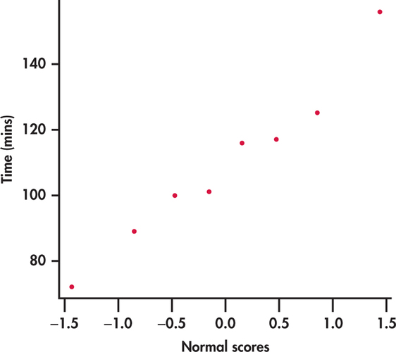
The use of the $t$ confidence interval in Example 7.1 rests on assumptions that appear reasonable here. First, we assume that our random sample is an SRS from the students at your institution. Second, because our sample size is not large, we assume that the distribution of times is Normal. With only eight observations, this assumption cannot be effectively checked. We can, however, check if the data suggest a severe departure from Normality. Figure 7.2 shows the Normal quantile plot, and we can clearly see there are no outliers or severe skewness. Deciding whether to use the $t$ confidence interval for inference about $μ$ is often a judgment call. We provide some practical guidelines to assist in this decision later in this section.

Apply Your Knowledge

Question 7.3

7.3 More on apartment rents.

Refer to Exercise 7.1 (page 360). Construct a 95% confidence interval for the mean monthly rent of all advertised one-bedroom apartments.

7.3

(655.528, 750.472).

Question 7.4

7.4 90% versus 95% confidence interval.

If you chose 90%, rather than 95%, confidence in the previous exercise, would your margin of error be larger or smaller? Explain your answer.

The one-sample $t$ test

Significance tests of the mean $μ$ using the standard error of $\bar{x}$ are also very similar to the $z$ test described in the last chapter. We still carry out the four steps required to do a significance test, but because we use $s$ in place of $σ$ , the distribution we use to find the $P$ -value changes from the standard Normal to a $t$ distribution. Here are the details.

Reminder

$z$ significance test, p. 327

One-Sample $t$ Test

Suppose that an SRS of size $n$ is drawn from a population having unknown mean $μ$ . To test the hypothesis $H_{0} : μ = μ_{0}$ , compute the one-sample $t$ statistic

$t = \frac{\bar{x} - μ_{0}}{s / \sqrt{n}}$

Page 363

In terms of a random variable $T$ having the $t (n - 1)$ distribution, the $P$ -value for a test of $H_{0}$ against

$H_{a} : μ > μ_{0} is P (T \geq t)$

$H_{a} : μ < μ_{0} is P (T \leq t)$

$H_{a} : μ \neq μ_{0} is 2 P (T \geq | t |)$

These $P$ -values are exact if the population distribution is Normal and are approximately correct for large $n$ in other cases.

EXAMPLE 7.2 Does the Average Amount of Time Using a Smartphone at Your Institution Differ from the UK Average?

smrtphn

CASE 7.1 Can the results of the Samsung and $O_{2}$ be generalized to the population of students at your institution? To help answer this, we can use the SRS in Example 7.1 (page 361) to test whether the average time using a smartphone at your institution differs from the UK average of 119 minutes. Specifically, we want to test

$\begin{array}{l} H_{0} : μ = 119 \\ H_{a} : μ \neq 119 \end{array}$

at the 0.05 significance level. Recall that $n = 8, \bar{x} = 109.5$ , and $s = 25.33$ . The $t$ test statistic is

$\begin{array}{l} t = \frac{\bar{x} - μ_{0}}{s / \sqrt{n}} & = \frac{109.5 - 119}{25.33 / \sqrt{8}} \\ = - 1.06 \end{array}$

This means that the sample mean $\bar{x} = 109.5$ is slightly more than one standard error below the null hypothesized value of 119.

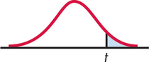
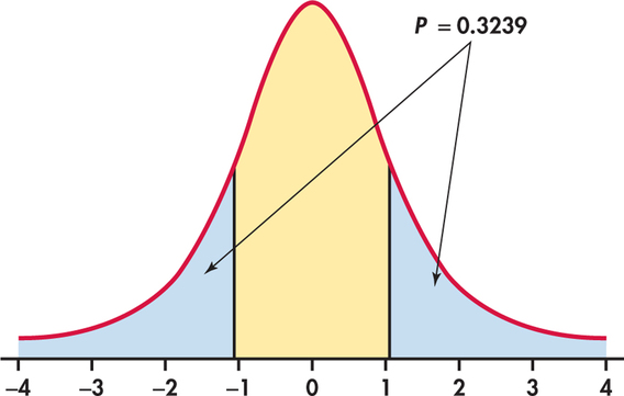
Because the degrees of freedom are $n - 1 = 7$ , this $t$ statistic has the $t (7)$ distribution. Figure 7.3 shows that the $P$ -value is $2 P (T \geq | - 1.06 |)$ , where $T$ has the $t (7)$ distribution. From Table D, we see that $P (T \geq 0.896) = 0.20$ and $P (T \geq 1.119) = 0.15$ .

Therefore, we conclude that the $P$ -value is between $2 \times 0.15 = 0.30$ and $2 \times 0.20 = 0.40$ . Software gives the exact value as $P = 0.3239$ . These data are compatible with an average of $μ = 119$ minutes per day. Under $H_{0}$ , a difference this large or larger would occur about one time in three simply due to chance. There is not enough evidence to reject the null hypothesis at the 0.05 level.

$df = 7$
$p$	0.20	0.15
$t^{*}$	0.896	1.119

Page 364

FIGURE 7.3 Sketch of the

$P$ -value calculation, Example 7.2.

In this example, we tested the null hypothesis $μ = 119$ against the two-sided alternative $μ \neq 119$ . Because we had suspected that the average time would be smaller, we could have used a one-sided test.

EXAMPLE 7.3 One-sided Test for Average Time Using a Smartphone

smrtphn

CASE 7.1 To test whether the average amount of time using a smartphone is less than the UK average our hypotheses are

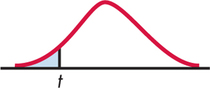
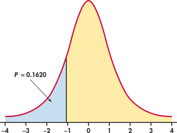
$\begin{array}{l} H_{0} : μ = 119 \\ H_{a} : μ < 119 \end{array}$

The $t$ test statistic does not change: $t = - 1.06$ . As Figure 7.4 illustrates, however, the $P$ -value is now $P (T \leq - 1.06)$ , half of the value in Example 7.2. From Table D, we can determine that $0.15 < P < 0.20$ ; software gives the exact value as $P = 0.1620$ . Again, there is not enough evidence to reject the null hypothesis in favor of the alternative at the 0.05 significance level.

FIGURE 7.4 Sketch of the

$P$ -value calculation, Example 7.3.

Page 365

For these data, our conclusion does not depend on the choice between a one-sided and a two-sided alternative hypothesis. Sometimes, however, this choice will affect the conclusion, and so this choice needs to be made prior to analysis. It is wrong to examine the data first and then decide to do a one-sided test in the direction indicated by the data. If in doubt, always use a two-sided test. This is the alternative hypothesis to use when there is no prior suspicion that the mean is larger or smaller.

Apply Your Knowledge

Question 7.5

7.5 Apartment rents.

Refer to Exercise 7.1 (page 360). Do these data give good reason to believe that the average rent for all advertised one-bedroom apartments is greater than $650 per month? Make sure to state the hypotheses, find the $t$ statistic, degrees of freedom, and $P$ -value, and state your conclusion using the 5% significance level.

7.5

$H_{0} : μ = $ 650. H_{a} : μ > $ 650, t = 2.30, d f = 24, 0.01 < P -value < 0.02$ . There is enough evidence to believe that the average rent for all advertised one-bedroom apartments is greater than $650 per month at the 0.05 significance level.

Question 7.6

7.6 Significant?

A test of a null hypothesis versus a two-sided alternative gives $t = 2.25$ .

The sample size is 13. Is the test result significant at the 5% level? Explain how you obtained your answer.
The sample size is 9. Is the test result significant at the 5% level?
Sketch the two $t$ distributions to illustrate your answers.

Question 7.7

7.7 Average quarterly return.

A stockbroker determines the short-run direction of the market using the average quarterly return of stock mutual funds. He believes the next quarter will be profitable when the average is greater than 1%. He will get complete quarterly return information soon, but right now he has data from a random sample of 30 stock funds. The mean quarterly return in the sample is 1.5%, and the standard deviation is 1.9%. Based on this sample, test to see if the broker will feel the next quarter will be profitable.

State appropriate null and alternative hypotheses. Explain how you decided between the one- and two-sided alternatives.
Find the $t$ statistic, degrees of freedom, and $P$ -value. State your conclusion using the $α = 0.05$ significance level.

7.7

(a) $H_{0} : μ = 1 % . H_{a} : μ > 1 %$ . Because the next quarter will be profitable when the average is greater than 1%, this indicates a one-sided alternative. (b) $t = 1.44, d f = 29, 0.05 < P -value<0 .10$ . The data do not give good evidence that the next quarter will be profitable.

Using software

For small data sets, such as the one in Example 7.1 (page 361), it is easy to perform the computations for confidence intervals and significance tests with an ordinary calculator and Table D. For larger data sets, however, software or a statistical calculator eases our work.

EXAMPLE 7.4 Diversify or Be Sued

divrsfy

An investor with a stock portfolio worth several hundred thousand dollars sued his broker and brokerage firm because lack of diversification in his portfolio led to poor performance. The conflict was settled by an arbitration panel that gave “substantial damages” to the investor.² Table 7.1 gives the rates of return for the 39 months that the account was managed by the broker. The arbitration panel compared these returns with the average of the Standard & Poor’s 500-stock index for the same period.

Page 366

Table 7.4: TABLE 7.1 Monthly rates of return on a portfolio (percent)

−8.36	1.63	−2.27	−2.93	−2.70	−2.93	−9.14	−2.64
6.82	−2.35	−3.58	6.13	7.00	−15.25	−8.66	−1.03
−9.16	−1.25	−1.22	−10.27	−5.11	−0.80	−1.44	1.28
−0.65	4.34	12.22	−7.21	−0.09	7.34	5.04	−7.24
−2.14	−1.01	−1.41	12.03	−2.56	4.33	2.35

Consider the 39 monthly returns as a random sample from the population of monthly returns that the brokerage would generate if it managed the account forever. Are these returns compatible with a population mean of $μ = 0.95 %$ , the S&P 500 average? Our hypotheses are

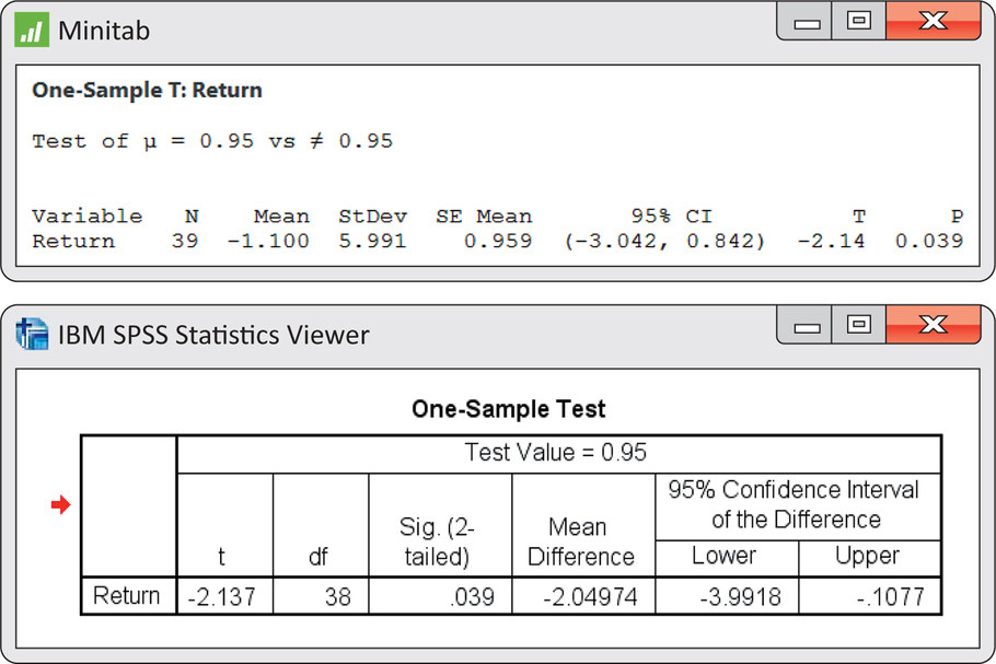
$\begin{array}{l} H_{0} : μ = 0.95 \\ H_{a} : μ \neq 0.95 \end{array}$

Figure 7.5 gives a histogram for these data. There are no outliers, and the distribution shows no strong skewness. We are reasonably confident that the distribution of $\bar{x}$ is approximately Normal, and we proceed with our inference based on Normal theory. Minitab and SPSS outputs appear in Figure 7.6. Output from other software will look similar.

FIGURE 7.5 Histogram of monthly rates of return for a stock portfolio, Example 7.4.

FIGURE 7.6 Minitab and SPSS outputs, Examples 7.4 and 7.5.

Page 367

Here is one way to report the conclusion: the mean monthly return on investment for this client’s account was $\bar{x} = - 1.1 %$ . This differs significantly from 0.95, the performance of the S&P 500 for the same period $(t = - 2.14, df = 38, P = 0.039)$

The hypothesis test in Example 7.4 leads us to conclude that the mean return on the client’s account differs from that of the stock index. Now let’s assess the return on the client’s account with a confidence interval.

EXAMPLE 7.5 Estimating Mean Monthly Return

divrsfy

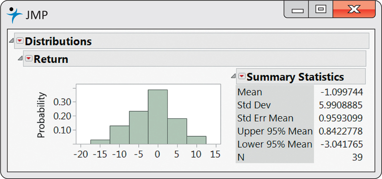
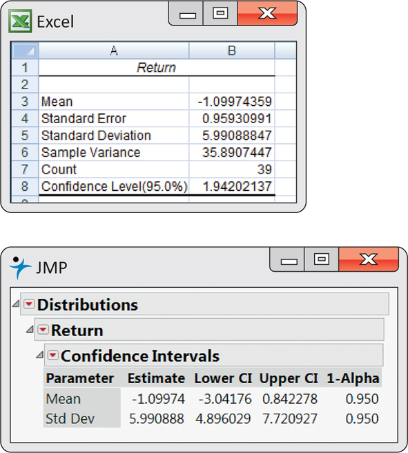
The mean monthly return on the client’s portfolio was $\bar{x} = - 1.1 %$ , and the standard deviation was $s = 5.99 %$ . Figure 7.6 gives the Minitab and SPSS outputs, and Figure 7.7 gives the Excel and JMP outputs for a 95% confidence interval for the population mean $μ$ . Note that Excel gives the margin of error next to the label “Confidence Level(95.0%)” rather than the actual confidence interval. We see that the 95% confidence interval is (−3.04, 0.84), or (from Excel) $- 1.0997 \pm 1.9420$ .

FIGURE 7.7 Excel and JMP outputs, Example 7.5.

Because the S&P 500 return, 0.95%, falls outside this interval, we know that $μ$ differs significantly from 0.95% at the $α = 0.05$ level. Example 7.4 gave the actual $P$ -value as $P = 0.039$ .

The confidence interval suggests that the broker’s management of this account had a long-term mean somewhere between a loss of 3.04% and a gain of 0.84% per month. We are interested not in the actual mean but in the difference between the broker’s process and the diversified S&P 500 index.

Page 368

EXAMPLE 7.6 Estimating Difference from a Standard

divrsfy

Following the analysis accepted by the arbitration panel, we are considering the S&P 500 monthly average return as a constant standard. (It is easy to envision scenarios in which we would want to treat this type of quantity as random.) The difference between the mean of the investor’s account and the S&P 500 is $\bar{x} - μ = - 1.10 - 0.95 = - 2.05 %$ . In Example 7.5, we found that the 95% confidence interval for the investor’s account was (−3.04,0.84). To obtain the corresponding interval for the difference, subtract 0.95 from each of the endpoints. The resulting interval is (−3.04−0.95, 0.84−0.95), or (−3.99, −0.11). This interval is presented in the SPSS output of Figure 7.6. We conclude with 95% confidence that the underperformance was between −3.99% and −0.11%. This estimate helps to set the compensation owed to the investor.

Apply Your Knowledge

Question 7.8

CASE 7.1

7.8 Using software to compute a confidence interval.

In Example 7.1 (page 360), we calculated the 95% confidence interval for the average daily time a student at your institution uses his or her smartphone. Use software to compute this interval, and verify that you obtain the same interval.

smrtphn

Question 7.9

CASE 7.1

7.9 Using software to perform a significance test.

In Example 7.2 (page 360), we tested whether the average time per day of a student using a smartphone was different from the UK average. Use software to perform this test and obtain the exact $P$ -value.

smrtphn

Matched pairs $t$ procedures

The smartphone use problem of Case 7.1 concerns only a single population. We know that comparative studies are usually preferred to single-sample investigations because of the protection they offer against confounding. For that reason, inference about a parameter of a single distribution is less common than comparative inference.

Reminder

confounding, p. 143

One common comparative design, however, makes use of single-sample procedures. In a matched pairs study, subjects are matched in pairs and the outcomes are compared within each matched pair. For example, an experiment to compare two marketing campaigns might use pairs of subjects that are the same age, sex, and income level. The experimenter could toss a coin to assign the two campaigns to the two subjects in each pair. The idea is that matched subjects are more similar than unmatched subjects, so comparing outcomes within each pair is more efficient (that is, reduces the standard deviation of the estimated difference of treatment means). Matched pairs are also common when randomization is not possible. For example, before-and-after observations on the same subjects call for a matched pairs analysis.

Reminder

matched pairs design, p. 154

EXAMPLE 7.7 The Effect of Altering a Software Parameter

The MeasureMind® 3D MultiSensor metrology software is used by various companies to measure complex machine parts. As part of a technical review of the software, researchers at GE Healthcare discovered that unchecking one option reduced measurement time by 10%. This time reduction would help the company’s productivity provided the option has no impact on the measurement outcome. To investigate this, the researchers measured 76 parts using the software both with and without this option checked.³

Page 369

Table 7.5: TABLE 7.2 Parts measurements using optical software

Part	OptionOn	OptionOff	Diff	Part	OptionOn	OptionOff	Diff
1	118.63	119.01	0.38	11	119.03	118.66	−0.37
2	117.34	118.51	1.17	12	118.74	118.88	0.14
3	119.30	119.50	0.20	13	117.96	118.23	0.27
4	119.46	118.65	−0.81	14	118.40	118.96	0.56
5	118.12	118.06	−0.06	15	118.06	118.28	0.22
6	117.78	118.04	0.26	16	118.69	117.46	−1.23
7	119.29	119.25	−0.04	17	118.20	118.25	0.05
8	120.26	118.84	−1.42	18	119.54	120.26	0.72
9	118.42	117.78	−0.64	19	118.28	120.26	1.98
10	119.49	119.66	0.17	20	119.13	119.15	0.02

geparts

Table 7.2 gives the measurements (in microns) for the first 20 parts. For analysis, we subtract the measurement with the option on from the measurement with the option off. These differences form a single sample and appear in the “Diff” columns for each part.

To assess whether there is a difference between the measurements with and without this option, we test

$\begin{array}{l} H_{0} : μ = 0 \\ H_{a} : μ \neq 0 \end{array}$

Here $μ$ is the mean difference for the entire population of parts. The null hypothesis says that there is no difference, and $H_{a}$ says that there is a difference, but does not specify a direction.

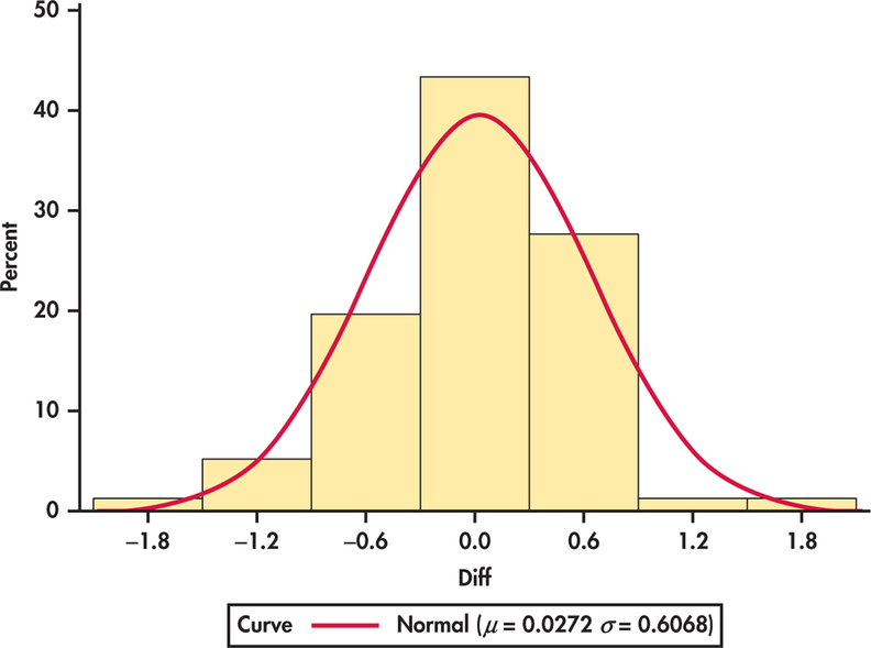
The 76 differences have

$\bar{x} = 0.027 and s = 0.607$

Figure 7.8 shows a histogram of the differences. It is reasonably symmetric with no outliers, so we can comfortably use the one-sample $t$ procedures. Remember to always check assumptions before proceeding with statistical inference.

FIGURE 7.8 Histogram of the differences in measurements (option off minus option on), Example 7.7.

Page 370

The one-sample $t$ statistic is

$\begin{array}{l} t = \frac{\bar{x} - 0}{s / \sqrt{n}} & = \frac{0.027}{0.607 / \sqrt{76}} \\ = 0.39 \end{array}$

The $P$ -value is found from the $t (75)$ distribution. Remember that the degrees of freedom are 1 less than the sample size.

Table D does not provide a row for 75 degrees of freedom, but for both $t (60)$ and $t (80), t = 0.39$ lies to the left of the first column entry. This means the $P$ -value is greater than $2 (0.25) = 0.50$ . Software gives the exact value $P = 0.6967$ . There is little evidence to suggest this option has an impact on the measurements. When reporting results, it is usual to omit the details of routine statistical procedures; our test would be reported in the form: “The difference in measurements was not statistically significant $(t = 0.39, df = 75, P = 0.70)$ .”

This result, however, does not fully address the goal of this study. A lack of statistical significance does not prove the null hypothesis is true. If that were the case, we would simply design poor experiments whenever we wanted to prove the null hypothesis. The more appropriate method of inference in this setting is to consider equivalence testing. With this approach, we try to prove that the mean difference is within some acceptable region around 0. We can actually perform this test using a confidence interval.

equivalence testing

EXAMPLE 7.8 Are the Two Means Equivalent?

geparts

Suppose the GE Healthcare researchers state that a mean difference less than 0.25 microns is not important. To see if the data support a mean difference within $0.00 \pm 0.25$ microns, we construct a 90% confidence interval for the mean difference.

The standard error is

${SE}_{\bar{x}} = \frac{s}{\sqrt{n}} = \frac{0.607}{\sqrt{76}} = 0.070$

so the margin of error is

$m = t^{*} \times {SE}_{\bar{x}} = (1.671) (0.070) = 0.116$

where the critical value $t^{*} = 1.617$ comes from Table D using the conservative choice of 60 degrees of freedom.

$df = 60$
$t^{*}$	1.671	2.000
$C$	90%	95%

The confidence interval is

$\begin{array}{l} \bar{x} \pm m & = 0.027 \pm 0.116 \\ = (- 0.089, 0.143) \end{array}$

This interval is entirely within the $0.00 \pm 0.25$ micron region that the researchers state is not important. Thus, we can conclude at the 95% confidence level that the two means are equivalent. The company can turn this option off to save time obtaining measurements.

If the resulting 90% confidence interval would have been outside the stated region or contained values both within and outside the stated region, we would not have been able to conclude that the means are equivalent.

Page 371

One Sample Test of Equivalence

Suppose that an SRS of size $n$ is drawn from a population having unknown mean $μ$ . To test, at significance level $α$ , if $μ$ is within a range of equivalency to $μ_{0}$ , specified by the interval $μ_{0} \pm δ$ :

Compute the confidence interval with $C = 1 - 2 α$ .
Compare this interval with the range of equivalency.

If the confidence interval falls entirely within $μ_{0} \pm δ$ , conclude that $μ$ is equivalent to $μ_{0}$ . If the confidence interval is outside the equivalency range or contains values both within and outside the range, conclude the $μ$ is not equivalent to $μ_{0}$ .

Apply Your Knowledge

Question 7.10

7.10 Oil-free deep fryer.

Researchers at Purdue University are developing an oil-free deep fryer that will produce fried food faster, healthier, and safer than hot oil.⁴ As part of this development, they ask food experts to compare foods made with hot oil and their oil-free fryer. Consider the following table comparing the taste of hash browns. Each hash brown was rated on a 0 to 100 scale, with 100 being the highest rating. For each expert, a coin was tossed to see which type of hash brown was tasted first.

	Expert
	1	2	3	4	5
Hot Oil	78	83	61	71	63
Oil free	75	85	67	75	66

Is there a difference in taste? State the appropriate hypotheses, and carry out a matched pairs $t$ test using $α = 0.05$ .

Question 7.11

7.11 95% confidence interval for the difference in taste.

To a restaurant owner, the real question is how much difference there is in taste. Use the preceding data to give a 95% confidence interval for the mean difference in taste scores between oil-free and hot-oil frying.

7.11

$(- 1.77, 6.57)$

Robustness of the one-sample $t$ procedures

The matched pairs $t$ procedures use one-sample $t$ confidence intervals and significance tests for differences. They are, therefore, based on an assumption that the population of differences has a Normal distribution. For the histogram of the 76 differences in Example 7.7 shown in Figure 7.8 (page 369), the data appear to be slightly skewed. Does this slight non-Normality suggest that we should not use the $t$ procedures for these data?

All inference procedures are based on some conditions, such as Normality. Procedures that are not strongly affected by violations of a condition are called robust. Robust procedures are very useful in statistical practice because they can be used over a wide range of conditions with good performance.

Robust Procedures

A statistical inference procedure is called robust if the probability calculations required are insensitive to violations of the conditions that usually justify the procedure.

Page 372

The condition that the population be Normal rules out outliers, so the presence of outliers shows that this condition is not fulfilled. The $t$ procedures are not robust against outliers, because $\bar{x}$ and $s$ are not resistant to outliers.

Fortunately, the $t$ procedures are quite robust against non-Normality of the population, particularly when the sample size is large. The $t$ procedures rely only on the Normality of the sample mean $\bar{x}$ . This condition is satisfied when the population is Normal, but the central limit theorem tells us that a mean $\bar{x}$ from a large sample follows a Normal distribution closely even when individual observations are not Normally distributed.

Reminder

central limit theorem, p. 294

To convince yourself of this fact, use the $t$ Statistic applet to study the sampling distribution of the one-sample $t$ statistic. From one of three population distributions, 10,000 SRSs of a user-specified sample size $n$ are generated, and a histogram of the $t$ statistics is constructed. You can then compare this estimated sampling distribution with the $t (n - 1)$ distribution. When the population distribution is Normal, the sampling distribution is always $t$ distributed. For the other two distributions, you should see that as $n$ increases, the histogram looks more like the $t (n - 1)$ distribution.

To assess whether the $t$ procedures can be used in practice, Normal quantile plots, stemplots, histograms, and boxplots are all good tools for checking for skewness and outliers. For most purposes, the one-sample $t$ procedures can be safely used when $n \geq 15$ unless an outlier or clearly marked skewness is present. In fact, the condition that the data are an SRS from the population of interest is the more crucial assumption, except in the case of small samples. Here are practical guidelines, based on the sample size and plots of the data, for inference on a single mean:⁵

Sample size less than 15: Use $t$ procedures if the data are close to Normal. If the data are clearly non-Normal or if outliers are present, do not use $t$ .
Sample size at least 15: The $t$ procedures can be used except in the presence of outliers or strong skewness.
Large samples: The $t$ procedures can be used even for clearly skewed distributions when the sample is large, roughly $n \geq 40$ .

For the measurement study in Example 7.7 (pages368–370), there is only slight skewness and no outliers. With $n = 76$ observations, we should feel comfortable that the $t$ procedures give approximately correct results.

Apply Your Knowledge

Question 7.12

7.12 Significance test for the average time to start a business?

Consider the sample of time data presented in Figure 1.30 (page 54). Would you feel comfortable applying the $t$ procedures in this case? Explain your answer.

Question 7.13

7.13 Significance test for the average T-bill interest rate?

Consider data on the T-bill interest rate presented in Figure 1.29 (page 53). Would you feel comfortable applying the $t$ procedures in this case? Explain your answer.

7.13

Yes, although the data is strongly skewed, $n \geq 40$ implies we can still use the t procedure.

BEYOND THE BASICS: The Bootstrap

Confidence intervals and significance tests are based on sampling distributions. In this section, we have used the fact that the sampling distribution of $\bar{x}$ is $N (μ, σ / \sqrt{n})$ when the data are an SRS from an $N (μ, σ)$ population. If the data are not Normal, the central limit theorem tells us that this sampling distribution is still a reasonable approximation as long as the distribution of the data is not strongly skewed and there are no outliers. Even a fair amount of skewness can be tolerated when the sample size is large.

Page 373

What if the population does not appear to be Normal and we have only a small sample? Then we do not know what the sampling distribution of $\bar{x}$ looks like. The bootstrap is a procedure for approximating sampling distributions when theory cannot tell us their shape.⁶

bootstrap

The basic idea is to act as if our sample were the population. We take many samples from it. Each of these is called a resample. We calculate the mean $\bar{x}$ for each resample. We get different results from different resamples because we sample with replacement. Thus, an observation in the original sample can appear more than once in a resample. We treat the resulting distribution of $\bar{x}$ ’s as if it were the sampling distribution and use it to perform inference. If we want a 95% confidence interval, for example, we could use the middle 95% of this distribution.

resample

EXAMPLE 7.9 Bootstrap Confidence Interval

smrtphn

Consider the eight time measurements (in minutes) spent using a smartphone in Example 7.1 (page 361):

117

156

116

125

101

100

We defended the use of the one-sided $t$ confidence interval for an earlier analysis. Let’s now compare those results with the confidence interval constructed using the bootstrap.

We decide to collect the $\bar{x}$ ’s from 1000 resamples of size $n = 8$ . We use software to do this very quickly. One resample was

116

100

116

156

125

100

with $\bar{x} = 109.25$ . The middle 95% of our 1000 $\bar{x}$ ’s runs from 93.125 to 128.003. We repeat the procedure and get the interval (93.872, 125.750).

The two bootstrap intervals are relatively close to each other and are more narrow than the one-sample $t$ confidence interval (88.3,130.7). This suggests that the standard $t$ interval is likely a little wider than it needs to be for these data.

The bootstrap is practical only when you can use a computer to take a large number of samples quickly. It is an example of how the use of fast and easy computing is changing the way we do statistics.