The distribution of populations is limited to ecologically suitable habitats

As we have seen in previous chapters, the natural world varies from place to place. At the beginning of this chapter we saw that collared lizards inhabited habitat patches, known as glades, interspersed within a forest. As these glades were invaded by cedar trees, however, they became less suitable for the collared lizards. In this section, we will explore how ecologists determine the suitability of habitats. We will see that understanding habitat suitability is critical for understanding where a species is capable of living and the extent to which a species can expand its geographic range.

Determining Suitable Habitats

In Chapter 1, we mentioned that a species niche includes the range of abiotic and biotic conditions it can tolerate. We are now ready to elaborate on this point. To explore the concept of niche, scientists find it useful to draw a distinction between the fundamental niche and the realized niche of a species.

The fundamental niche of a species is the range of abiotic conditions under which species can persist. This includes the range of temperature, humidity, and salinity conditions that allow a population to survive, grow, and reproduce.

Although a species can potentially live under the conditions of its fundamental niche, many favorable locations can remain unoccupied because of other species in those locations. For example, the presence of competitors, predators, and pathogens can often prevent a population from persisting in an area, despite the existence of favorable abiotic conditions. The range of abiotic and biotic conditions under which a species persists is its realized niche. The realized niche determines the geographic range of a species or of various populations that compose a species. The geographic range is a measure of the total area covered by a population. For example, the American chestnut tree (Castanea dentata) was once a very common tree in the eastern forest of the United States because it grew and reproduced well under the abiotic and biotic conditions that existed in this region for thousands of years. Around 1900, however, a fungus (Cryphonectria parasitica) introduced from Asia caused a deadly disease known as chestnut blight. The fungus spread rapidly throughout the eastern forests and killed billions of trees. As a result of this biotic interaction between the chestnut trees and the fungus, few places remain where adult trees can persist. In short, the fungus has caused a major reduction in the realized niche of the American chestnut.

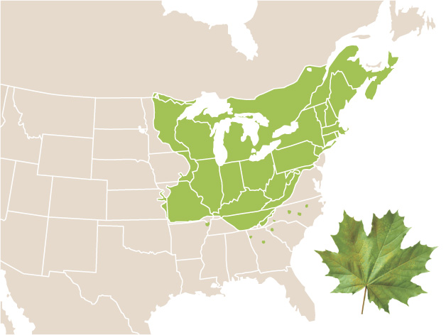
When we think about the geographic range of a species or population, we need to realize that individuals often do not occupy every location within the range. This is because climate, topography, soils, vegetation structure, and other factors influence the abundance of individuals. Consider the case of the sugar maple tree. As shown in Figure 11.1, its geographic range includes the midwestern United States, the northeastern United States, and southeastern Canada. Its distribution is limited by cold winter temperatures at the northern extent of its range, by summer droughts at the western extent, and by hot summer temperatures at the southern extent. Throughout this entire range, however, the sugar maple does not live everywhere. For instance, it cannot live in marshes, newly formed sand dunes, recently burned areas, and a variety of other habitats that lie outside its fundamental niche. As a result, the geographic range of the sugar maple is actually composed of a patchwork of smaller occupied and unoccupied areas.

Figure 11.1 The geographic range of the sugar maple. The range is limited in the north by low winter temperatures, to the south by high summer temperatures, and to the west by droughts.

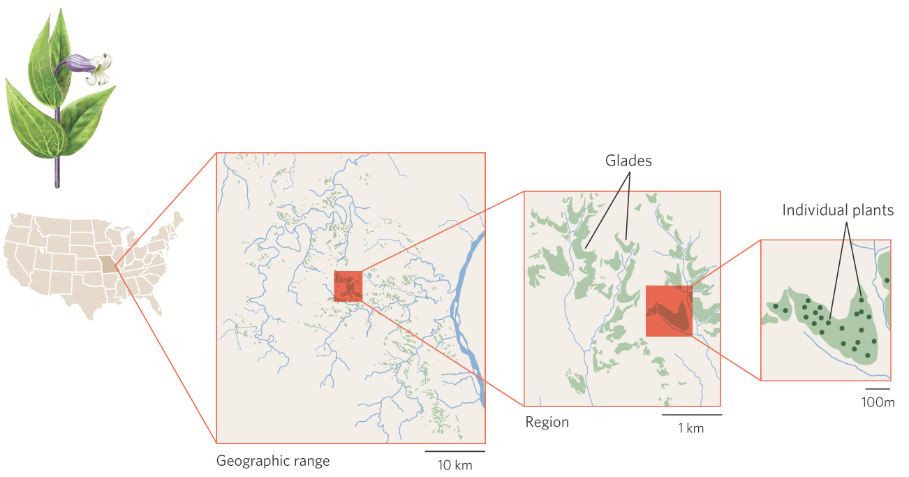
The distribution of a shrub known as Fremont’s leather flower (Clematis fremontii) provides an excellent example of how small-scale variation in the environment can create geographic ranges that are composed of small patches of suitable habitat. As illustrated in Figure 11.2, a survey of the plant’s geographic range in 1945 found that it was restricted to just three counties in the state of Missouri. This small range is thought to be the result of climatic conditions and competitive interactions with ecologically similar plants. Within its geographic range, the plant is restricted to dry, rocky soils on outcroppings of limestone, known as limestone glades, which are similar to the glades frequented by the collared lizard discussed at the beginning of this chapter. Small variations in elevation and soil quality further confine these plants within each limestone glade to sites with suitable soil structure, moisture, and nutrients. Local aggregations occurring on each of these sites consist of individuals that are fairly evenly distributed in space. In other words, while Fremont’s leather flower has a geographic range that includes three counties, its distribution is spotty in this region due to its narrow habitat requirements.

Figure 11.2 The geographic range of Fremont’s leather flower. A 1945 survey found that this shrub species was only found in three counties in the state of Missouri. Within this range, individuals were only found living in outcroppings of limestone, known as glades.

Data from R. O. Erickson, The Clematis fremontii var. Reihlii population in the Ozarks, Annals of the Missouri Botanical Garden 32 (1945): 413–460.

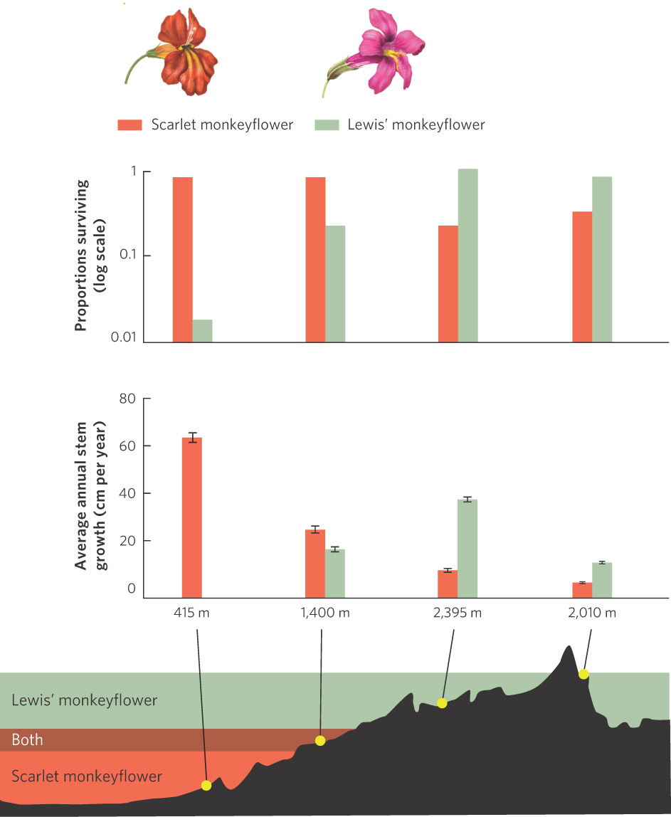
Although patterns of distribution would suggest that only certain habitats are suitable, we can test whether this is the case. In a recent experiment, investigators observed that two species of wildflowers lived at distinct elevations in the Sierra Nevada of California. One species, known as Lewis’ monkeyflower (Mimulus lewisii), lives at higher elevations. The other species, known as the scarlet monkeyflower (Mimulus cardinalis), lives at lower elevations. Both species occur at mid-elevations. To determine if the environmental conditions caused these different species distributions, researchers planted the two species at locations within and outside of the elevations where they grow in nature. The results of this experiment are shown in Figure 11.3. If we examine plant survival, we see that Lewis’ monkeyflower survives well at high elevations but survives poorly at low elevations. The opposite is true for the scarlet monkeyflower. If we examine plant growth, a similar pattern emerges. Lewis’ monkeyflower grows better as elevation increases, although growth declines under the extreme conditions of the highest elevation. The scarlet monkeyflower grows the best at low elevations and its growth declines with each increase in elevation. For each species, the survival and growth of the transplanted populations were the highest when grown within its normal elevation range. When grown outside this range, both species experienced lower survival and slower growth.

Figure 11.3 The distribution of two monkeyflower species. The scarlet monkeyflower is found at low elevations whereas Lewis’ monkeyflower grows at high elevations, as shown in the cross-section of the mountain. When transplanted to gardens at different elevations, the scarlet monkeyflower survives best at low elevations while Lewis’ monkeyflower survives best at high elevations. Similar patterns occur for plant growth. Error bars are standard errors.

Data from A. L. Angert and D. W. Schemske, The evolution of species’ distributions: Reciprocal transplants across the elevation ranges of Mimulus cardinalis and M. lewisii, Evolution 59 (2005): 1671–1684.

Ecological Niche Modeling

As a general rule, the more suitable the habitat, the larger a population can grow. This fundamental relationship between the environment and the distribution of populations allows ecologists to predict the actual or potential distributions of species. This predictive ability has a number of important applications. For example, when biologists wish to bring species back from the brink of extinction, they need to know the habitat conditions that the species requires. With this knowledge, biologists can determine the locations that would provide the highest probability of successful reintroductions. Similarly, if a new pest species is accidentally introduced to a continent, biologists can assess what habitat might be suitable and predict the area over which it might spread. This allows biologists to predict the extent of the damage it might cause.

Predicting the potential geographic range of a single population or of all populations of a given species is a major challenge when there are few individuals living in the wild. One way researchers have overcome this challenge is by using historic data on the distributions of populations. Such data are often available from collections of preserved organisms stored in museums and herbariums. In addition, when species have been introduced from other continents, researchers can try to determine the suitable habitat conditions found on the originating continent.

The process of determining the suitable habitat conditions for a species is known as ecological niche modeling. Because temperature and precipitation have a dominant influence on the distribution of biomes, modelers often begin by mapping the known locations of a species and then by quantifying the ecological conditions at the locations where the species has been recorded. The modeler can potentially include many additional variables such as different soil types and the presence of potential predators, competitors, and pathogens that might limit the population’s distribution. The range of ecological conditions that are predicted to be suitable for a species is the ecological envelope of the species. The concept of the ecological envelope is similar to the realized niche, but the realized niche includes the conditions under which a species currently lives whereas the ecological envelope is a prediction of where a species could potentially live. Using the conditions in the ecological envelope, the modeler can determine what other locations in a region have the same ecological conditions and therefore might serve as additional suitable habitat.

Modeling the Spread of Invasive Species

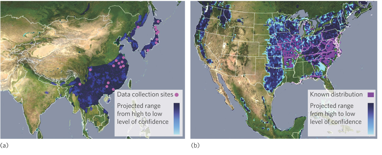
Ecological niche modeling can be a useful way to predict the expansion of pest species introduced to a continent where they have not previously lived. One example is the Chinese bushclover (Lespedeza cuneata), which is native to eastern Asia. In the late 1800s, this species of bushclover was brought to North Carolina to help control erosion, reclaim land that had been mined, and provide food for cattle. Over time, though, the plant quickly spread into the Great Smoky Mountains National Park and throughout the grasslands of the United States where it displaces native plants. To determine the likely extent of its future spread, ecologists gathered data on the environmental conditions under which the bushclover lived in 28 locations in Asia. As illustrated in Figure 11.4a, they then quantified the ecological envelope for the clover to predict the entire geographic range in Asia. They used this data to successfully predict the potential geographic range in North America. As you can see in Figure 11.4b, they predicted all locations where the clover has already spread. The model also predicts that the clover has the potential to live in many other locations, with widespread negative effects on the plant communities. The fact that not all of these predicted areas have Chinese bushclover in them yet suggests either that there are additional ecological factors important to the clover and not included in the model or that the clover simply has not had enough time to disperse to these more distant locations.

Figure 11.4 Ecological modeling of an invasive species. (a) Researchers collected data on the environmental conditions where the Chinese bushclover lives in Asia and used these data to predict the entire native range of the plant in Asia. (b) They then used the data to predict the future geographic range of Chinese bushclover in North America, where the plant was introduced 100 years ago and has continued to spread slowly.

Data from A. T. Peterson et al., Predicting the potential invasive distributions of four alien plant species in North America, Weed Science 51 (2003): 863–868.

Habitat Suitability and Global Warming

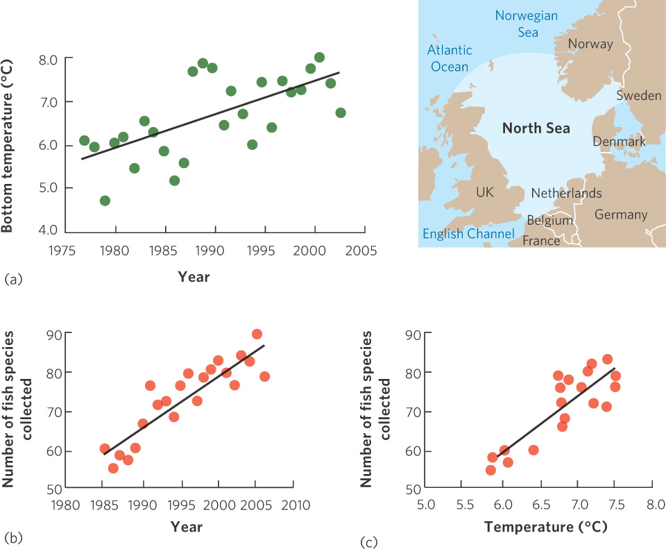
Knowledge of the environmental conditions that make a habitat suitable can also be used to understand the shift in the geographic ranges of species as the environmental conditions of the world change. During the past century, for example, the average temperature of Earth has increased by 0.8°C. Some regions of the world—such as Alaska and northern Canada—have warmed as much as 4°C. In the relatively shallow North Sea, situated between the United Kingdom and Norway, temperatures in the bottom waters have increased 0.7°C per decade since the 1970s. As shown in Figure 11.5a, this translates to a 2°C increase in temperature from 1977 to 2003. Given that most species of fish have optimal temperature ranges, we might predict that warming ocean waters could cause southern fish species, which live in warm waters, to move north.

Figure 11.5 Changes in the distribution of fish in the North Sea. (a) From 1977 to 2003, the temperature of the water at the bottom of the North Sea increased by 2°C. (b) Surveys of fish trawls from 1985 to 2006 found that the total number of fish species collected per year in the North Sea increased from 60 to approximately 90. (c) The total number of fish species collected per year was positively correlated with the average sea temperatures during the previous 5 years.

Data from J. G. Hiddink and R. ter Hofstede, Climate induced increases in species richness of marine fishes, Global Change Biology 14 (2008): 453–460.

During the same period that temperatures in the North Sea were being monitored, the International Council for the Exploration of the Sea (ICES) compiled data on fish distributions by pulling large nets (called “trawls”) along the ocean floor. From 1985 to 2006, scientists from six countries worked together to fish the bottom of the ocean at 300 locations distributed throughout the North Sea. Based on 7,000 trawl samples, the researchers reported in 2008 that fish species richness in the North Sea had increased steadily over 22 years. As you can see in Figure 11.5b, there were about 60 species in the mid-1980s but this grew to nearly 90 species 2 decades later. This list of species included dozens of more southerly species that had expanded their ranges northward.

The increase in species richness was positively correlated with the increase in bottom-water temperatures in the North Sea. This correlation—shown in Figure 11.5c—suggests that warmer temperatures are more hospitable to a greater variety of species, and that the warming of the North Sea has allowed more southerly species to expand the northern edges of their ranges into the area. Hence, this is a case of global warming increasing the diversity of species in a region.

The increase in the diversity of species in the North Sea not only is dramatically changing the fish community but also may affect the important commercial fisheries that depend on this community. For example, the three species whose ranges have contracted as the North Sea became warmer—the wollfish (Anarhichas lupus), the spurdog (Squalus acanthias), and the ling (Molva molva)—are all commercially important, whereas more than half of the southerly species with expanded ranges have little or no commercial value. As a result, while these shifts in species distributions with warming temperatures may increase fish diversity, it could actually decrease the value of North Sea commercial fisheries.