Populations have growth limits
In nature we commonly observe that there are limits on how large a population can grow. Ecologists categorize these limits as being either density independent or density dependent. In this section we will review these two types of limits on population growth and discuss how we can incorporate them into population growth models.
Density-Independent Factors
Density independent Factors that limit population size regardless of the population’s density.
As the name suggests, density-independent factors limit population size regardless of the population’s density. Common density-independent factors include natural disasters such as tornadoes, hurricanes, floods, and fires. However, other less dramatic changes in the environment, including extreme temperatures and droughts, can also limit populations. In all of these cases, the impact on the population is not related to the number of individuals in the population. Consider, for example, what happens when a hurricane hits a coastal forest. The number of trees that survive the hurricane is independent of the number of trees that were present before the hurricane arrived.
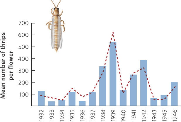
A classic study on density-independent effects was conducted by James Davidson and Herbert Andrewartha in Australia during the 1930s and 1940s. The apple thrip (Thrips imaginis) was a common insect pest in Australia that would occasionally increase to very large numbers and devastate apple trees and rose bushes throughout large regions of the country. From 1932 to 1946, the researchers surveyed thrip populations on rose bush flowers in an attempt to understand the causes of the large variations in population size. They suspected that these population changes were the result of density-independent factors such as seasonal variation in temperature and rainfall. Figure 12.5 shows the population sizes the researchers predicted and the population sizes they observed. As you can see, the predicted changes in thrip abundance closely matched the actual number of thrips they counted in their surveys.
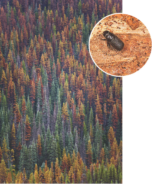
Understanding the role of density-independent factors remains an important goal of ecologists today. For example, in 2011 researchers from the U.S. Forest Service and the Canadian Forest Service reported on the impacts of bark beetles in western North America. Bark beetles are native insects that consume the phloem tissues of trees, causing them to die. During the past several decades, bark beetles have killed billions of coniferous trees covering millions of hectares from Mexico to Alaska (Figure 12.6). Under warmer temperatures, bark beetles develop faster and have more generations per year, but they can be killed by unusually cold temperatures. As a result, temperature is a major determinant of population size. Concerned about the possible effect of climate change on the population of bark beetles, researchers looked at expectations for increased climate warming and applied their knowledge of bark beetle ecology to project future growth. They concluded that bark beetle populations are likely to increase dramatically and cause more damage to conifer trees in the future.
277
Density-Dependent Factors
Density dependent Factors that affect population size in relation to the population’s density.
Density-dependent factors affect population size in relation to the population’s density. Ecologists find it useful to break these factors down into two categories. Negative density dependence occurs when the rate of population growth decreases as population density increases. Positive density dependence, also known as inverse density dependence, occurs when the rate of population growth increases as population density increases. Because positive density dependence was first proposed by the ecologist Warder Allee in 1931, it is also known as the Allee effect.
Negative density dependence When the rate of population growth decreases as population density increases.
Positive density dependence When the rate of population growth increases as population density increases. Also known as inverse density dependence or the Allee effect.
Some of the most common negative density-dependent factors include resources that are available in limited supply, such as food, nesting sites, and physical space. When a population is small, there is an abundance of resources for all individuals, but as the population increases, such resources are divided among more individuals. As a result, the per capita amount of resources declines and at some point it reaches a level at which individuals find it difficult to grow, reproduce, and survive. This was the concern Malthus expressed in the eighteenth century about the rapid growth of the human population.
Although competition for food is a common challenge for populations that grow to large sizes, it is not the only challenge. Crowded populations also can have higher levels of stress, transmit diseases at a greater rate, and attract the attention of predators. All of these factors can act to slow, and finally halt, population growth.
Negative Density Dependence in Animals
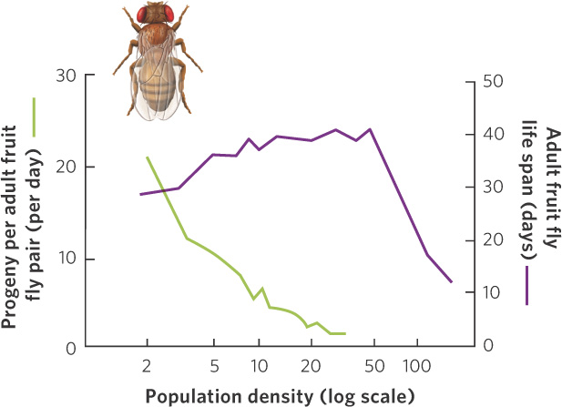
In a classic experiment that investigated density-dependent regulation of populations, Raymond Pearl introduced pairs of fruit flies (Drosophila melanogaster) at different densities into laboratory bottles containing identical amounts of food. As the number of individuals in the bottles increased, competition for food became more intense and the number of progeny produced per pair of adult flies decreased, as shown in Figure 12.7. With even larger populations, the life span of the adults also sharply declined, demonstrating that both the young and old fruit flies were affected by the competition for food.
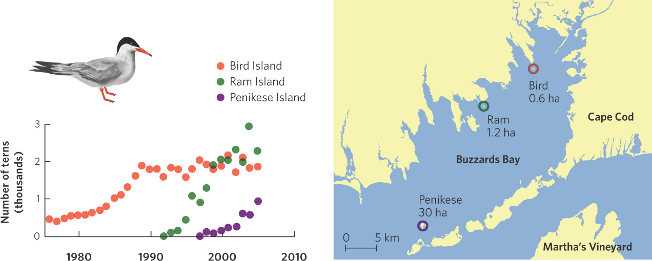
Although negative density dependence is easily demonstrated in the laboratory, a number of natural experiments have confirmed the existence of the phenomenon in nature. For example, the common tern (Sterna hirundo) is a bird that nests on beaches. In the 1970s, the tern population on the eastern coast of North America began to expand into an area known as Buzzards Bay in Massachusetts. It first colonized Bird Island where its numbers quickly grew from about 200 to 1,800 individuals by 1990, as shown in Figure 12.8. For these terns the factor limiting population growth appears to be the availability of suitable nesting sites. By 1991, most suitable breeding sites on Bird Island were occupied and the population leveled off. The following year, birds began to colonize Ram Island, where the population increased to just over 2,000 birds and then leveled off by the year 2000. Around this time, the terns began to colonize Penikese Island. These data demonstrate that although the terns have a high intrinsic growth rate, a limited number of nesting sites ultimately limits the population size.
278
Negative Density Dependence in Plants
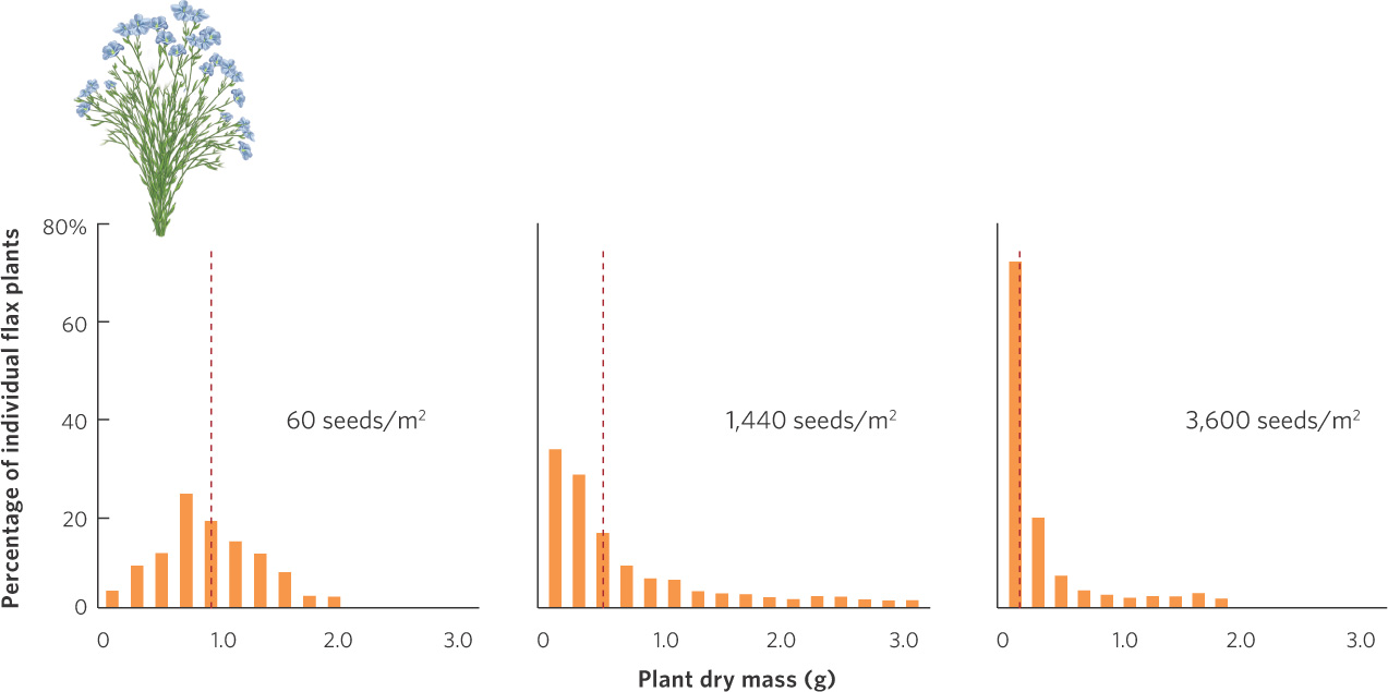
Plants also experience reduced fecundity and increased mortality at high densities. When plants are grown at high densities, each plant has access to fewer resources such as sunlight, water, and soil nutrients. As a result, it is harder for each plant to grow. We can see this outcome in a study of flax plants (Linum usitatissimum) that were grown at a wide range of densities and then dried to determine their mass. The data from this experiment are shown in Figure 12.9. When seeds were sown at a density of 60 seeds per m2, the average dry weight of individuals was between 0.5 and 1 g. When seeds were sown at densities of 1,440 and 3,600 per m2, most of the individuals weighed less than 0.5 g. Plants with reduced growth typically experience reduced fecundity. As a result, the high competition caused by high plant densities will cause a population of flax plants to grow more slowly.
Under very high densities, competition among conspecifics can cause plants to die. In an experiment using horseweed (Erigeron canadensis), seeds were sown at a density of 100,000 per m2. Competition among the tiny seedlings was intense; as you can see in Figure 12.10a, over an 8-month period most of them died. A close examination of the two y axes in the figure illustrates that there was a hundredfold decrease in population density but a thousandfold increase in the average weight of the surviving individuals. As a result, the total mass of the plants increased tenfold over time.
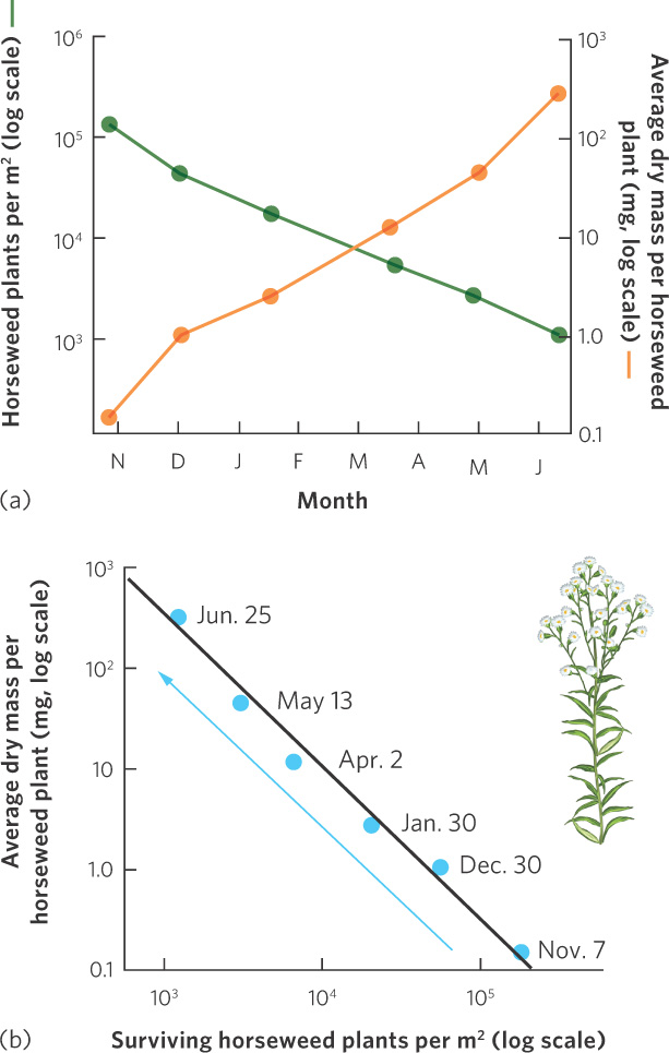
Self-thinning curve A graphical relationship that shows how decreases in population density over time lead to increases in the size of each individual in the population.
In Figure 12.10b, you can see the same data, but now we have graphed the density of surviving plants over time against the average dry mass per plant, using a log scale. When we graph these data, we see that the data fall on a line with a slope of approximately  . Plant ecologists call this relationship a self-thinning curve. This relationship has been observed frequently across a wide variety of species. The insights that emerge from the self-thinning curve have a number of practical uses. For example, the curve can be used to predict survival and growth of crop plants that might be sown at different densities in agricultural fields or the growth and survival of tree seedlings that might be planted at different densities in forest plantations.
In plants, animals, and other taxonomic groups, negative density dependence tends to bring populations under control and to maintain their abundances at a level close to the maximum number that can be supported by the environment. In many cases, populations are affected by density-independent and density-dependent factors. Next we consider the fascinating process of positive density dependence.
Positive Density Dependence
Whereas negative density dependence causes population growth to decrease as population density increases, positive density dependence causes population growth to increase as population density increases. Positive density dependence typically occurs when population densities are very low and can be caused by several different mechanisms. In some cases, very low densities make it hard for individuals to find mates or, in the case of flowering plants, to obtain pollen, which can reduce reproductive success and slow population growth. Very low densities can also lead to the harmful effects of inbreeding, as discussed in Chapter 4. There can also be problems associated with small population sizes that, by chance, have uneven sex ratios. Small populations with a low proportion of females can suffer low population growth rates. Finally, individuals living in smaller populations can face a higher predation risk than those living in large populations, as we discussed in Chapter 10. In short, while negative density dependence causes slow population growth due to overcrowding, positive density dependence causes slow population growth due to undercrowding.
279
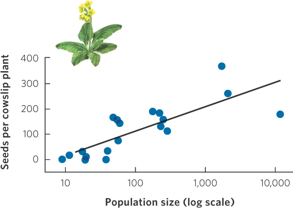
Positive density dependence has been demonstrated in a wide variety of species. Many plant species, for example, avoid the costs of inbreeding through a number of mechanisms that prevent self-fertilization. They depend on receiving pollen from other plants, but this can be difficult when individuals live at low densities and are widely spread over an area. In a study of cowslip (Primula veris), a plant of European grasslands, researchers were interested in determining why many of the smaller populations were declining. When they looked at reproduction in populations of different sizes, they found that populations of fewer than 100 individuals produced fewer seeds per plant, as can be seen in Figure 12.11. This probably occurred because the small populations were not as good at attracting pollinators and plants received less pollen.
280
A recent study found that positive density dependence also occurs in parasites. In 2012, researchers reported on reproduction in salmon lice (Lepeophtheirus salmonis), which feed on the skin of salmon. When breeding, male and female lice form a mating pair. Researchers in British Columbia counted the number of mating pairs on each fish and found that the probability of an individual forming a mating pair was positively correlated with the number of lice of the opposite sex. Individuals living at low densities have a hard time finding a mate and therefore the lice experienced positive density dependence.
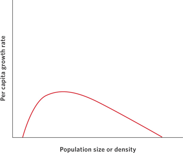
Although we often think of positive and negative density dependence as isolated phenomena, populations can be regulated by both processes, as shown in Figure 12.12. As we move from low densities to intermediate densities, the effects of positive dependence play an important role. Increased densities provide more individuals for breeding and the growth rate of the population can improve. Above some intermediate density, resources start to become limiting and negative density dependence begins to play a role. As densities continue to increase, negative density dependence continues to slow population growth and, eventually, the population growth rate falls to zero.
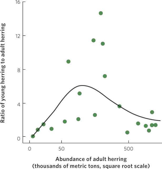
An example of the dynamic between positive and negative effects of density on population growth can be found in a population of herring (Clupea harengus) that spawns near Iceland. As you can see in Figure 12.13, the herring experience low population growth at low densities, high population growth at intermediate densities, and then a return to low population growth at high densities. The existence of positive density dependence in the herring population concerns fisheries managers because it indicates that if the herring were driven to low densities by fishing, it would be difficult for the population to bounce back. In fact, the populations could experience negative growth rates and become extinct. Fortunately, most fish populations do not appear to experience positive density dependence.
281
The herring study highlights why those who manage populations in the wild need to understand positive density dependence. For example, when a species has declined to very low numbers and we wish to improve its numbers, management strategies need to consider how to avoid inbreeding and how to ensure that each female can encounter a sufficient number of mates to fertilize all of her eggs. The concept of positive density dependence also offers an opportunity for ecologists to help control undesirable pest species. For example, several pest insects have been controlled by releasing sterile males into the population. This skews the sex ratio and causes the females to breed with sterile males, leading to a lower growth rate in the pest population. In other cases, researchers have simply reduced the size of an undesirable population to the point that individuals have a hard time finding mates.
The Logistic Growth Model
Carrying capacity (K) The maximum population size that can be supported by the environment.
Although positive and negative density dependence both occur in nature, the effects of negative density dependence have received much more attention from population modelers. Researchers have developed population growth models that mimic the behavior of many natural populations: rapid initial growth followed by slower growth as populations grow toward their maximum size. The maximum population size that can be supported by the environment is known as the carrying capacity of the population, denoted as K.
To model the slowing growth of populations at high densities, we use the logistic growth model. The logistic growth model builds on the exponential growth model, but we add a term in parentheses that accounts for a decline in growth rate as the population approaches its carrying capacity:
Logistic growth model A growth model that describes slowing growth of populations at high densities.
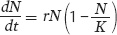
When the number of individuals in the population is small relative to the carrying capacity, the fraction  is close to 0 and the term inside the parentheses approaches 1. When this happens, the equation becomes nearly identical to the exponential growth model. However, when the number of individuals in the population approaches the carrying capacity, the term inside the parentheses approaches 0. As a result, the population’s rate of growth approaches 0. When we plot the growth of a population over time using the logistic growth curve, we obtain a sigmoidal, or S-shaped curve, which is shown in Figure 12.14. The middle point on the curve, where the population experiences its highest growth rate, is known as the inflection point. Above the inflection point, the population growth begins to slow.
S-shaped curve The shape of the curve when a population is graphed over time using the logistic growth model.
Inflection point The point on a sigmoidal growth curve at which the population achieves its highest growth rate.
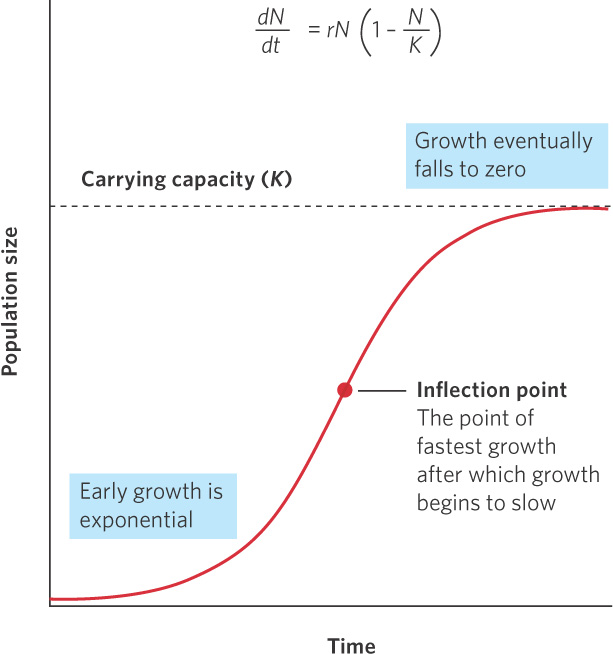
We can further understand how the logistic growth model behaves by examining the effect of population size on the rate of increase of the population  . As shown in Figure 12.15a, as the population increases from a very small size, the rate of increase grows because the number of reproductive individuals increases. After reaching one-half of the carrying capacity, which corresponds to the inflection point of the S-shaped curve, the rate of increase begins to slow because the reproductive individuals are each obtaining fewer resources.
282
We can also examine how population size affects the rate of increase on a per capita basis, which is:

As you can see in Figure 12.15b, individuals in the population continually decline in their ability to contribute to the growth of the population. These insights help us understand that the logistic growth curve shows an initial rapid increase in growth due to the increasing number of individuals in the population, followed by a slowing rate of growth as a large number of individuals experience limited per capita resources.
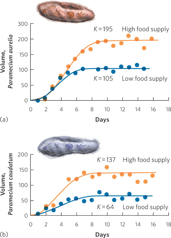
The logistic equation describes the growth of many populations. One of the classic studies was conducted by Russian biologist Georgyi Gause in 1934. Gause raised two species of protists, Paramecium aurelia and Paramecium caudatum, in test tubes and added a fixed amount of food each day. Both species initially experienced exponential growth, which then slowed until they reached carrying capacity. Because the two species differ in many ways, their populations stabilized at different carrying capacities, which are illustrated as blue lines in Figure 12.16. Gause suspected that the cause of this maximum population size was the amount of available food. To test this hypothesis, he did the experiment again, but this time doubled the amount of food. As you can see from the orange line in each graph, the two species once again experienced rapid initial growth followed by slower growth that stabilized. With twice as much food available, however, the two species stabilized at population sizes that were twice as large as in the first experiment. This early experiment confirmed that logistic growth can happen in real organisms and that the increased availability of a limiting resource can increase the carrying capacity of a population.
283
Predicting Human Population Growth With the Logistic Equation
The logistic growth model was first developed in 1838 by the Belgian mathematician Pierre François Verhulst. Verhulst had read Thomas Malthus’s 1798 essay and sought to formulate a natural law governing the growth of populations. Nearly a century later, in 1920, Raymond Pearl and Lowell Reed independently developed the logistic growth model when they examined human population growth in the United States.
Using census data that had been collected every 10 years, Pearl and Reed confirmed the observation by Malthus that the population in the United States initially grew exponentially from 1790 to 1910. They noticed, however, that by 1910 this growth began to slow, as illustrated in Figure 12.17, and that the rate of growth appeared to be declining over time. Based on these data, Pearl and Reed applied their logistic growth equation to the census data and predicted that the population of the United States, which was 91 million in 1910, had a carrying capacity of 197 million. However, they were careful to note that this prediction depended on the population supporting itself using only the land of the United States.
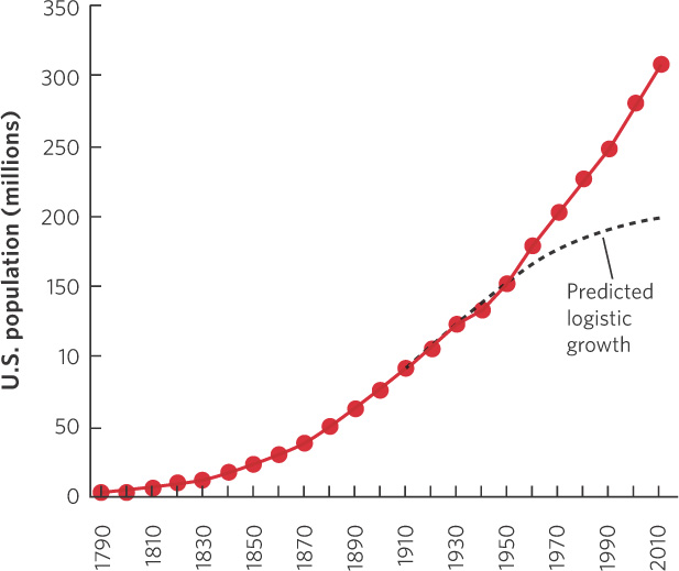
As you can see in the figure, the U.S. population has greatly exceeded this prediction; by 2012, the population was more than 310 million people. There are several reasons for this. One important reason is that technological advances have allowed farmers in the United States to produce food much more efficiently. Moreover, a substantial amount of the food consumed by the U.S. population comes from other regions of the world. In addition to the increases in available food, we have had major improvements in public health and medical treatment that have increased survival rates substantially, particularly for infants and children. Finally, the logistic equation did not incorporate the millions of immigrants that came to the United States after 1910.