Chance events can cause small populations to go extinct

In our models of population growth, we have seen that when populations are large, density-dependent factors cause slower growth, and when populations are small, density-dependent factors cause faster growth. Given these outcomes, it is hard to see how populations could go extinct, yet we know that extinction does occur in real populations in nature. In this section, we will explore the relationship between population size and the probability of extinction. We will then examine the underlying causes of this relationship.

Extinction in Small Populations

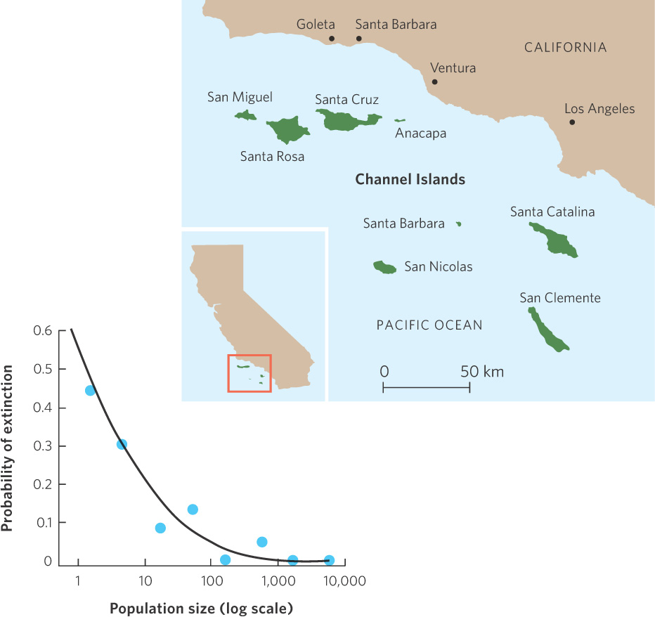
In nature we find that smaller populations are more vulnerable to extinction than larger populations. To study this phenomenon, biologists have conducted surveys of birds on the Channel Islands, which are located off the coast of California and range in size from 2.6 to 249 km². At different times over a period of approximately 80 years, researchers studied the number of breeding pairs of different species and the extinction rates of populations on particular islands. They categorized populations of species by size based on the number of breeding pairs they counted and then determined the extinction probability for populations of each size category. As shown in Figure 13.13, the smallest populations experienced the highest probability of extinction and the largest populations experienced the lowest probability of extinction. Similar patterns have been observed for many other groups of animals, including mammals, reptiles, and amphibians.

Figure 13.13 Smaller populations and the likelihood of extinction. Bird populations of the Channel Islands off the coast of California were measured in terms of the number of breeding pairs. Islands with larger population sizes had a reduced probability of going extinct over a period of 80 years.

Data from H. L. Jones and J. M. Diamond, Short-time-based studies of turnover in breeding bird populations on the California Channel Islands, Condor 78 (1976): 526–549.

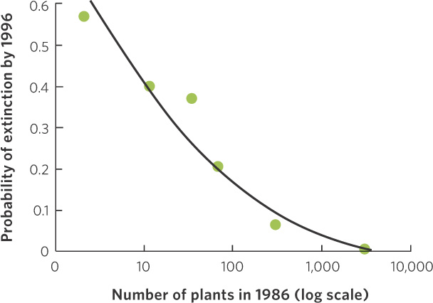
The increased extinction rate of small populations is also seen in plants. For example, researchers in Germany examined the persistence of 359 populations of plants that spanned eight different species. In 1986, they counted the number of individuals in each population and 10 years later found that 27 percent of the populations had gone extinct. As you can see in Figure 13.14, when the researchers placed the populations into one of six population sizes and averaged the extinction rates across the eight species, they found that the probability of extinction was high for smaller population sizes and low for larger populations.

Figure 13.14 The probability of plant populations going extinct. Researchers surveyed 359 plant populations in Germany in 1986 and then again in 1996. They then placed the populations into six size categories and averaged extinction rates across the eight species. They found that populations with the lowest number of individuals experienced the highest probability of extinction over a 10-year period.

Data from D. Matthies et al., Population size and the risk of local extinction: Empirical evidence from rare plants, Oikos 105 (2004): 481–488.

Extinction Due to Variation in Population Growth Rates

We have seen that populations are more likely to go extinct when they are small. However, the density-dependent population models we have examined show that small populations have more rapid growth rates than large populations. This suggests that a small population should quickly rebound and grow into a larger population. By this reasoning, small populations should be resistant to extinction. How do we resolve the fundamental difference between these models and our observations of actual populations?

The models that we have studied to this point have assumed a single birth rate and death rate for each individual in the population. When a model is designed to predict a result without accounting for random variation in population growth rate, we say it is a deterministic model. Although deterministic models are simpler to work with, not every individual in the real world has the same birth rate or the same probability of dying. Rather, because we see random variation among individuals in a population, the growth rate is not constant; it can vary over time. Models that incorporate random variation in population growth rate are known as stochastic models. When random variation in birth rates and death rates is due to differences among individuals and not due to changes in the environment, we call it demographic stochasticity. In contrast, when random variation in birth rates and death rates is due to changes in the environmental conditions, we call it environmental stochasticity. Examples of environmental stochasticity include changes in the weather, which can cause small changes in the growth rate of a population, and natural disasters, which can cause large changes in the growth rate of a population.

When we use stochastic models, there is an average growth rate with some variation around that average. The actual growth rate experienced by the modeled population can take any of the values within the range of this variation. As a result, a population’s growth rate may be above or below the average growth rate. If a population experiences a string of years with above average growth rates, it will have faster growth. If the population happens to have a string of years with below average growth rates, it will have slower growth. Which outcome actually occurs is determined strictly by chance.

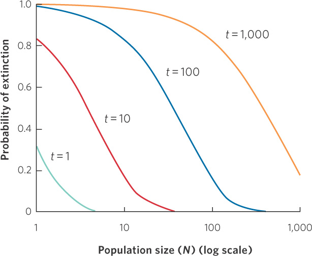
We can begin to account for stochasticity by adding it to the exponential growth model we discussed in Chapter 12. For example, we can set the birth rate and death rate to 0.5, which are reasonable values for adult mortality and recruitment in a population of terrestrial vertebrates. We can let populations vary above and below these average birth and death rates at random. When a population randomly experiences years of low birth rates or high death rates, it is more likely to go extinct. A string of bad years can drive the population extinct faster in small populations than in large populations. Moreover, at a given population size, as time passes there is an increased chance that a population will have a string of bad growth years and go extinct. You can see the effect of population size and time on the average probability of extinction in Figure 13.15. For example, in a population with 10 individuals, the average probability of extinction within 10 years is 0.16, the average probability of extinction within 100 years is 0.82, and extinction becomes virtually certain (0.98) within 1,000 years. In contrast, a population with an initial size of 1,000 has an average probability of extinction of only 0.18 within 1,000 years. By adding the reality of stochasticity to our population models, we see that although populations of any size eventually have some chance of going extinct, the smallest populations face the greatest risk of extinction.

Figure 13.15 The probability of extinction in a population model. Using an exponential growth model and stochastic rates of birth and death, the average probability of extinction increases with decreasing population sizes (N) and longer times into the future (t).