Populations of consumers and consumed populations fluctuate in regular cycles
In the previous chapter, we discussed how populations can fluctuate over time and space, and we saw that some populations experience population cycles. At the beginning of this chapter we introduced a study of population cycles for lynx and snowshoe hares. You can see the data from this study in Figure 14.7. The hare and lynx populations both experienced cycles of 9 to 10 years, with the lynx cycles lagging about 2 years behind the hare cycles.
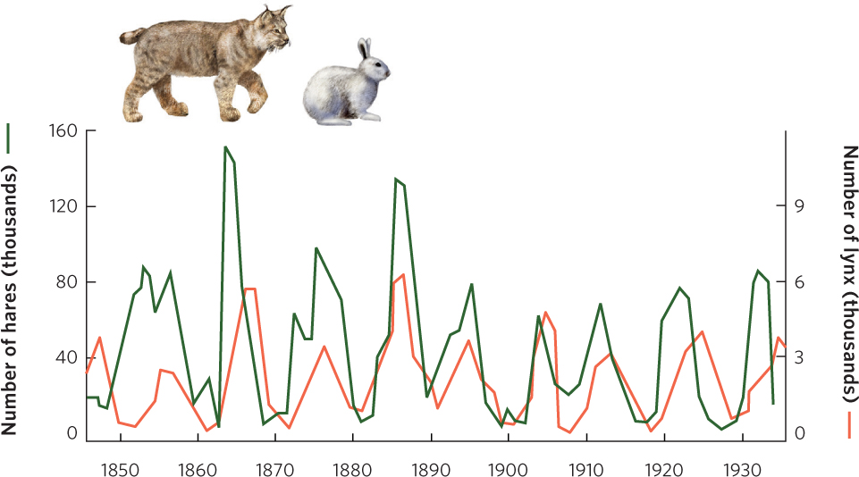
It turns out that other large herbivores in the boreal and tundra regions of Canada—such as muskrat, ruffed grouse, and ptarmigan—also have population cycles of 9 to 10 years. Smaller herbivores, such as voles, mice, and lemmings, tend to have 4-year cycles. Studies of predators in these regions have revealed that some predators—including red foxes, marten, mink, goshawks, and horned owls—feed on larger herbivores and have long population cycles. In contrast, other predators— including Arctic foxes (Vulpes lagopus), rough-legged hawks (Buteo lagopus), and snowy owls (Bubo scandiacus)—feed on small herbivores and have short population cycles. The close synchrony of population cycles between consumers and the populations they consume suggests that these oscillations are the result of interactions between them.
324
To understand the mechanisms underlying the predator–prey cycles, it is useful to examine them in the context of population models.
Creating Predator–Prey Cycles in the Laboratory
During the early twentieth century, biologists became interested in using predators and pathogens to control populations of crop and forest pests. One of the leading researchers in this effort was Carl Huffaker, a biologist at the University of California at Berkeley who pioneered the biological control of crop pests. Huffaker sought to understand the conditions that cause predator and prey populations to fluctuate. He chose two species of mites that lived on citrus trees: the six-spotted mite (Eotetranychus sexmaculatus) was the prey and the western predatory mite (Typhlodromus occidentalis) was the predator. In a series of experiments, he established populations on large trays that contained oranges—which were both habitat and food for the prey—with rubber balls interspersed among the oranges, as illustrated in Figure 14.8. On each tray, he varied the number and distribution of the oranges.
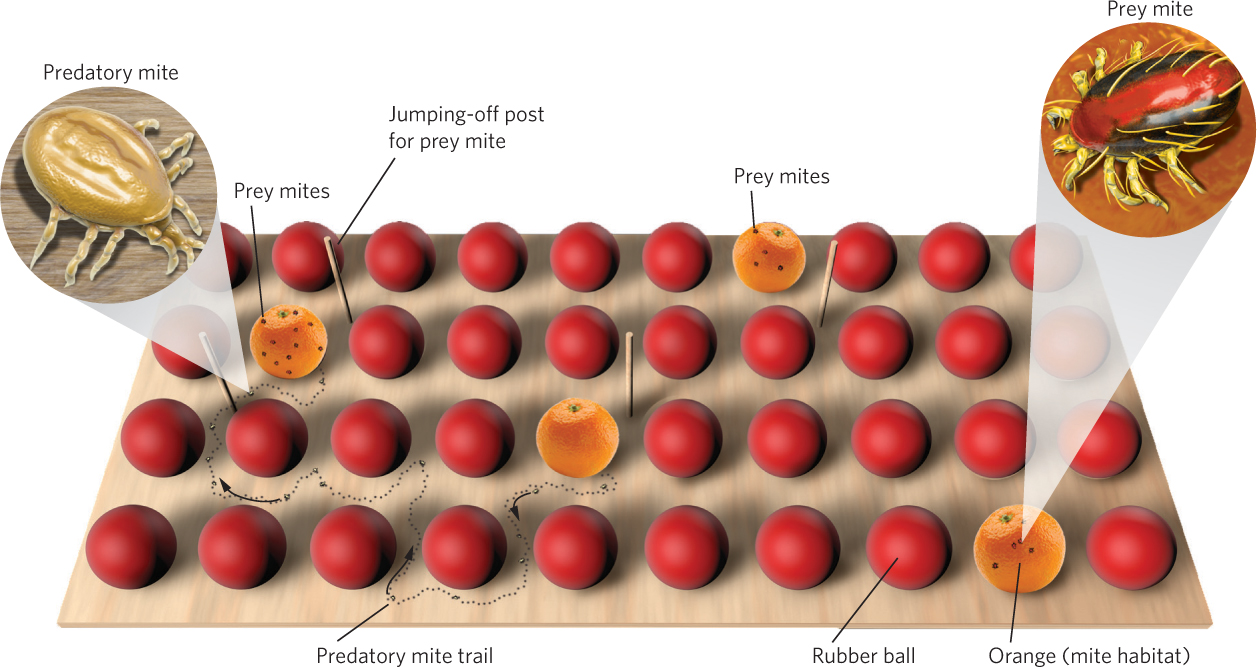
In most experiments, Huffaker initially added 20 female prey per tray and then introduced two female predators 11 days later; because both species reproduce parthenogenetically, no males were added. When the prey were introduced to trays without predators, the prey population leveled off at between 5,500 and 8,000 mites. When predators were added, the predator population increased rapidly and soon wiped out the prey population. Without prey to feed on, though, predators quickly became extinct. However, it took longer for predators and prey to go extinct if the oranges were spread far apart from each other because it took longer for the predators to locate the prey. In short, predators and prey could not coexist over time.
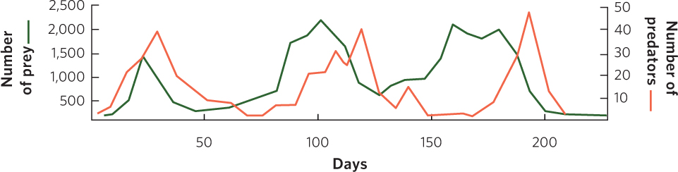
Huffaker reasoned that if predator dispersal could be further impeded, the two species might be able to coexist. To accomplish this, he introduced barriers to predator dispersal. The predatory mites disperse by walking, but the prey mites use a silk line that they spin to float on wind currents. Based on these differences, Huffaker modified his trays to give the prey a dispersal advantage by placing a mazelike pattern of Vaseline barriers among the oranges to slow the dispersal of the walking predators. He also placed vertical wooden pegs throughout the trays for the six-spotted mites to use as jumping-off points. This arrangement produced a series of three population cycles during the 8-month experiment, as depicted in Figure 14.9. The distribution of predators and prey throughout the trays continually shifted as the prey, which were on their way to extermination on one orange, recolonized another orange and stayed one step ahead of their predators. In short, Huffaker created a metapopulation in the laboratory.
325
Huffaker’s experiment demonstrated that predators and prey could not coexist in the absence of suitable refuges for the prey. However, the predator and prey populations were able to coexist through time in a spatial mosaic of suitable habitats that provided a dispersal advantage to the prey. Two kinds of time delays caused the populations to cycle: one was the result of predators dispersing more slowly between food patches than their prey, and the other was the result of time needed for predator numbers to increase through reproduction. From this we can conclude that stable population cycles can be achieved when the environment is complex enough that predators cannot easily find scarce prey.
Mathematical Models of Predator–Prey Cycles
Lotka-Volterra model A model of predator–prey interactions that incorporates oscillations in the abundances of predator and prey populations and shows predator numbers lagging behind those of their prey.
Even before Huffaker’s laboratory experiments on predator–prey cycles, mathematicians Alfred Lotka and Vito Volterra were developing models of predator–prey interactions. The Lotka-Volterra model incorporates oscillations in the abundances of predator and prey populations and shows predator numbers lagging behind those of their prey. It does this by calculating both the rate of change in the prey population and the rate of change in the predator population.
Let’s begin with the prey population. Following the convention of our population models in Chapter 12, we will designate the number of prey as N. We will then designate the number of predators as P. In words, the growth rate of the prey population depends on the rate of individuals being added to the prey population minus the rate of individuals being killed by predators:
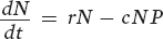
The first term in this equation (rN) represents the exponential growth of a prey population based on the intrinsic growth rate (r), as we saw in Chapter 12. For simplicity, this term does not include density dependence. The second term (cNP) represents the loss of individuals due to predation. The model assumes that the predation rate is determined by the probability of a random encounter between predators and prey (NP) and the probability of such an encounter leading to the prey’s capture (c) (think of c for “capture efficiency”).
Next we turn to the predator population. The equation for the predator population is similar to that for the prey population in that it has two terms, one term that represents the birth rate of the predator population and a second term that represents the death rate of the predator population:
The first term in the equation (acNP) represents the birth rate of the predator population. It is determined by the number of prey consumed by the predator population (cNP) multiplied by the efficiency of converting consumed prey into predator offspring (a). The second term (mP) represents the death rate of the predator population and is determined by the per capita mortality rate of predators (m) multiplied by the number of predators (P).
Changes in the Prey Population
We can use the Lotka-Volterra equations to determine the conditions that allow the prey population to be stable. By definition, a population is stable when its rate of change is zero. We can write this as:
0 = rN − cNP
326
We can rearrange this as:
rN = cNP
This indicates that the prey population becomes stable when the addition of prey (rN) is balanced by the consumption of prey (cNP). We can further simplify this equation as:
P = r ÷ c
This indicates that the prey population will be stable when the number of predators equals the ratio of the prey’s growth rate and the predator’s capture efficiency.
Now that we know the conditions that make the prey population stable, we can also explore the conditions that cause the prey population to increase or decrease. The prey population will increase when the addition of prey (rN) exceeds the consumption of prey (cNP), which we can write as:
rN > cNP
We can rearrange this inequality as:
P < r ÷ c
This inequality represents the number of predators that the population of prey can support and still increase. This number is higher when the growth potential of the prey population (r) is higher or when the predators are less efficient at capturing prey (c). Using the same logic, the prey population will decrease whenever
P > r ÷ c
Changes in the Predator Population
We can also use these equations to understand the conditions that make the predator population remain stable, increase, or decrease. Once again, the population is stable when the rate of change is zero:
0 = acNP − mP
We can rearrange this as:
acNP = mP
This indicates that the predator population becomes stable when the addition of predators (acNP) is balanced by the mortality of predators (mP). We can further simplify this equation as:
N = m ÷ ac
Given that this is the condition needed for a stable predator population, we can also determine the conditions required for predator populations either to increase or to decrease. The predator population will increase when the addition of predators exceeds the mortality of predators, which we can write as:
acNP > mP
We can rearrange this as:
N > m ÷ ac
This inequality represents the number of prey required to support the growth of the predator population. This number is higher when the death rate of predators (m) is higher, and it is lower when predators are more efficient at capturing prey (c) and converting them into offspring (a). Using the same logic, the predator population will decrease whenever
N < m ÷ ac
Trajectories of Predator and Prey Populations
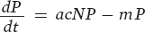
Knowing the conditions under which predator and prey populations increase, decrease, or remain stable helps us understand why predator and prey populations sometimes cycle. Figure 14.10a plots the abundance of both populations. We can draw a horizontal line at the point where P = r ÷ c, which is the number of predators associated with a stable prey population. This line is called the equilibrium isocline, or zero growth isocline, for the prey because it indicates the points at which a population is stable. At any combination of predator and prey numbers in the region below the equilibrium isocline, there are relatively few predators and the prey population increases. In the region above this line, the prey population decreases because predators remove them faster than they can reproduce.
Equilibrium isocline The population size of one species that causes the population of another species to be stable. Also known as Zero growth isocline.
We can also plot the equilibrium isocline for the predator population, as shown in Figure 14.10b. In this graph, we draw a vertical line at the point where N = m ÷ ac, which is the number of prey that causes the predator population to be stable. Any combination of predator and prey numbers that lies in the region to the right of this line allows the predator population to increase because there is an increased abundance of prey to consume. In the region to the left, the predator population decreases because there are not enough prey available.
Joint population trajectory The simultaneous trajectory of predator and prey populations.
We can now combine our understanding of how predator and prey populations change in abundance by considering the trajectory of both populations simultaneously, which we call a joint population trajectory.
327
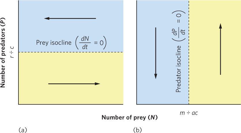
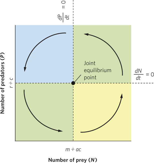
Figure 14.11 traces the path of the joint population trajectory. Beginning with the lower right region, predators and prey both increase, and their joint population trajectory moves up and to the right. In the upper right region, prey are still abundant enough that predators can increase, but the increasing number of predators depresses the prey population. Accordingly, the joint population trajectory moves up and to the left. In the upper left region, the continued decline in prey causes the predator population to decline, so the trajectory moves down and to the left. In the lower left region, the continued decline in predators allows the prey population to start increasing, which causes the trajectory to move down and to the right and completes the cycle. Together, the trajectories in the four regions define a counterclockwise cycling of predator and prey populations.
Joint equilibrium point The point at which the equilibrium isoclines for predator and prey populations cross.
At the center of Figure 14.11, you can see the joint equilibrium point, which is the point at which the equilibrium isoclines for predator and prey populations cross. The joint equilibrium point represents the combination of predator and prey population sizes that falls exactly at this point and will not change over time. If either of the populations strays from the joint equilibrium point, the populations will oscillate around the joint equilibrium point rather than returning to it.
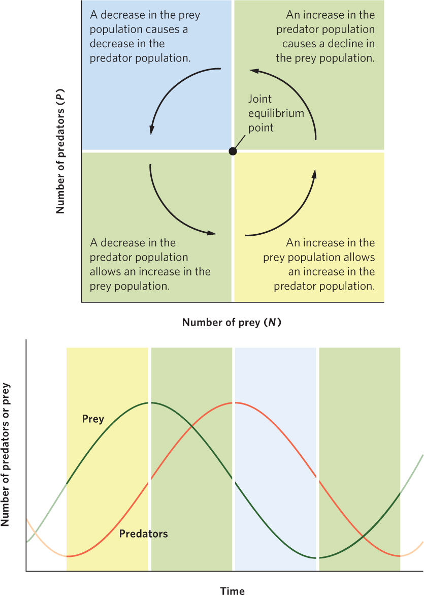
Based on the joint population trajectory of the Lotka-Volterra model, we can plot the changes in sizes of the two populations over time, as shown in Figure 14.12. This visualizes how the two populations cycle and reveals that the prey population remains one-fourth of a phase ahead of the predator population. Although some populations cycle due to time delays, as we discussed in Chapter 13, the predator–prey equations do not; the predator–prey equations are continuous equations in which population changes are immediate. Instead, the cycling is the result of each population responding to changes in the size of the other population. This pattern is reminiscent of the lynx population discussed at the beginning of this chapter that follows the fluctuations in the hare population.
328
Functional and Numerical Responses
The Lotka-Volterra model provides an explanation for population cycles that relies on a very simplified version of nature. As we have already discussed, it does not include time delays or density dependence, and it does not incorporate the real foraging behavior of most predators. To get a more realistic picture of predator and prey relationships, we have to consider the functional response and the numerical response of predators. As we will see, both of these responses help to stabilize the cycling of predator and prey populations.
329
The Functional Response
Functional response The relationship between the density of prey and an individual predator’s rate of food consumption.
The relationship between the density of prey and an individual predator’s rate of food consumption is known as the functional response of the predator. There are three potential categories of functional responses, as illustrated in Figure 14.13. For each of these categories, we can examine the number of prey consumed by each predator, shown in Figure 14.13a, or the proportion of prey consumed by each predator, shown in Figure 14.13b. A key point to remember is that whenever prey density increases and a predator can consume a higher proportion of those prey, the predator has the ability to regulate the growth of the prey population.
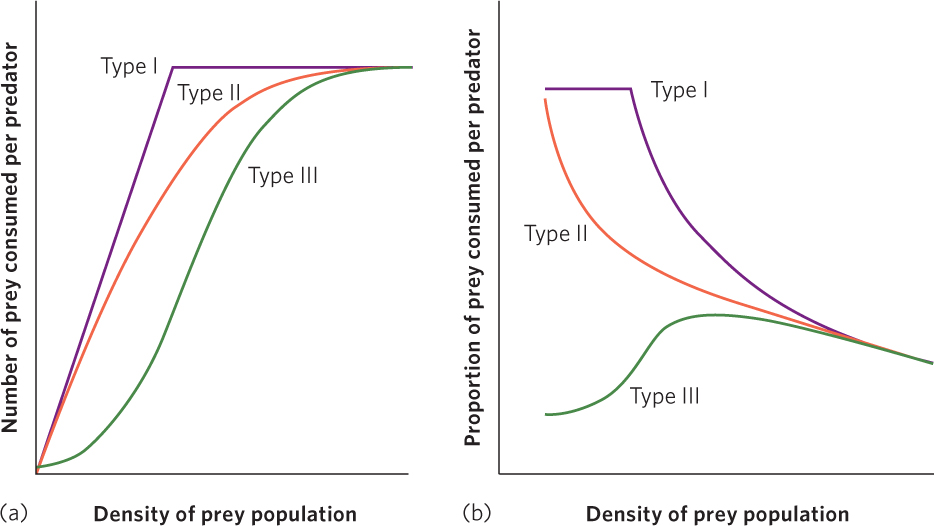
Type I functional response A functional response in which a predator’s rate of prey consumption increases in a linear fashion with an increase in prey density until satiation occurs.
A type I functional response, indicated by the purple line, occurs when a predator’s rate of prey consumption increases in a linear fashion with an increase in prey density until satiation occurs. As shown in Figure 14.13a, this means that increases in prey density result in an ever-increasing number of prey consumed by a predator until the predator becomes satiated and can consume no additional prey. Some species of predators, such as web-building spiders that catch an increasing number of prey as the density of prey increases, exhibit a type I functional response. As you can see in Figure 14.13b, this means that as prey density increases, each predator continues to consume a constant proportion of the prey up until the point of predator satiation. Once the prey become so dense that predator satiation occurs, the predators consume a continuously decreasing proportion of the prey. This is the functional response used by the Lotka-Volterra model that we discussed.
Type II functional response A functional response in which a predator’s rate of prey consumption begins to slow down as prey density increases and then plateaus when satiation occurs.
The type II functional response, shown by the orange line, occurs when the number of prey consumed slows as prey density increases and then plateaus when satiation occurs. The number of prey consumed slows because as predators consume more prey, they must spend more time handling the prey. For example, when a pelican catches a fish, it must take the time to manipulate the fish in its mouth and position the fish so that it will slide down the pelican’s throat. The more fish that the pelican catches, the more time it must spend handling fish, which leaves less time available to hunt for fish. Eventually, because the predator is spending so much of its time handling large numbers of fish and has little time remaining to catch additional fish, its predation rate levels off. In Figure 14.13b we can see that in a type II functional response any increases in prey density are associated with a slowing rate of prey consumption. As this occurs, the predators consume a smaller proportion of prey.
330
Type III functional response A functional response in which a predator exhibits low prey consumption under low prey densities, rapid consumption under moderate prey densities, and slowing prey consumption under high prey densities.
In a type III functional response, illustrated by the green line in Figure 14.13a, a predator exhibits low prey consumption under low prey densities, rapid consumption under moderate prey densities, and slowing prey consumption under high prey densities. Figure 14.13b shows how this type of functional response affects the proportion of prey consumed. As prey density increases there is an initial increase in the proportion of prey consumed. However, as the predators spend more time handling prey and become satiated, this proportion subsequently declines—just as we saw in the type II response.
Low consumption at low prey densities can be the result of three factors. First, at very low prey densities the prey can hide in refuges where they are safe from predators. A predator can consume prey only after the prey become so numerous that some individuals are unable to find a refuge.
Search image A learned mental image that helps the predator locate and capture food.
Second, at low prey densities predators have less practice locating and catching the prey, and therefore are relatively poor at doing it. As prey densities increase, however, the predators learn to locate and identify a particular species of prey, a phenomenon known as a search image. A search image is a learned mental image that helps the predator locate and capture food, just as a person might locate a can of cola in a grocery store by searching for a small, red cylinder.
A third factor that can cause relatively low consumption of prey at low densities is the phenomenon of prey switching. This occurs when one prey species is rare and a predator changes its preference to another prey species that is more abundant. If the first species then increases in density, the predator can switch back to it.
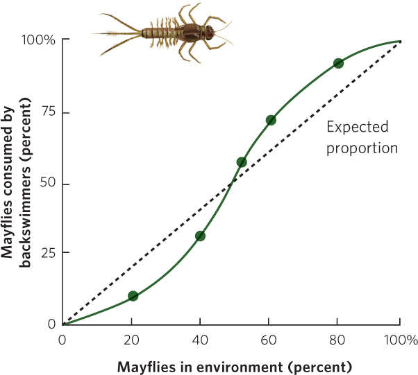
Many laboratory and field studies have demonstrated type III functional responses. For example, researchers examined the feeding preferences of a predatory insect known as a backswimmer (Notonecta glauca). Figure 14.14 shows what happened when the researchers presented the predator with two types of prey—isopods (Asellus aquaticus) and larval mayflies (Cloeon dipterum)—and manipulated the proportions of each prey species. If the predator could not develop a search image, it would consume the two prey species in proportion to their availability. If the predator could develop a search image, it would eat fewer than expected of the rare prey and more than expected of abundant prey. As predicted, when the mayflies were rare, the backswimmer consumed fewer mayflies than expected, given their abundance. When mayflies were abundant, however, the backswimmers consumed more mayflies than expected, based on their abundance.
331
The reason that the predator switched to the more abundant prey was because its success rate was higher with the prey that was present at high densities. For example, when larval mayflies were rare, predator attacks were successful less than 10 percent of the time. When the mayflies were common, predator attacks were successful nearly 30 percent of the time. Researchers attributed the improved capture rate to practice; the backswimmer became more proficient at catching the mayflies when it had more opportunities to catch them. The backswimmer exhibited no innate preference for either prey species, only a preference for the one that was more abundant.
The Numerical Response
Numerical response A change in the number of predators through population growth or population movement due to immigration or emigration.
As we have seen, the functional response considers changes in the number of prey consumed by each predator. A predator’s functional response helps us understand how many prey can be consumed by predators, and therefore the conditions under which predators can regulate prey populations. The numerical response is a change in the number of predators through population growth or population movement due to immigration or emigration. Populations of most predators usually grow slowly relative to populations of their prey, although the movement of mobile predators from surrounding areas can occur quite rapidly when the density of prey changes.
An example of numerical response occurs in local populations of the bay-breasted warbler (Dendroica castanea), a small insectivorous bird of eastern North America. During outbreaks of the spruce budworm, populations of the warbler increase dramatically. In most years, the warbler populations live at densities of about 25 breeding pairs per km2. However, during outbreak years, the warblers congregate in areas where the spruce budworm is living in high densities and warbler population densities can reach 300 breeding pairs per km2. As a result of this rapid numerical response, the predator has the potential to reduce prey densities quickly and to regulate the prey’s abundance.