Parasite and host populations commonly fluctuate in regular cycles

In our discussion of predators and prey in Chapter 14, we saw that population fluctuations are common and sometimes occur in regular cycles. Because parasites and hosts represent consumers and resources, they show similar population dynamics. In this section, we will examine how parasites and hosts fluctuate over time. We will also look at a mathematical model that helps us describe and understand the behavior of infectious pathogens and hosts.

Population Fluctuations in Nature

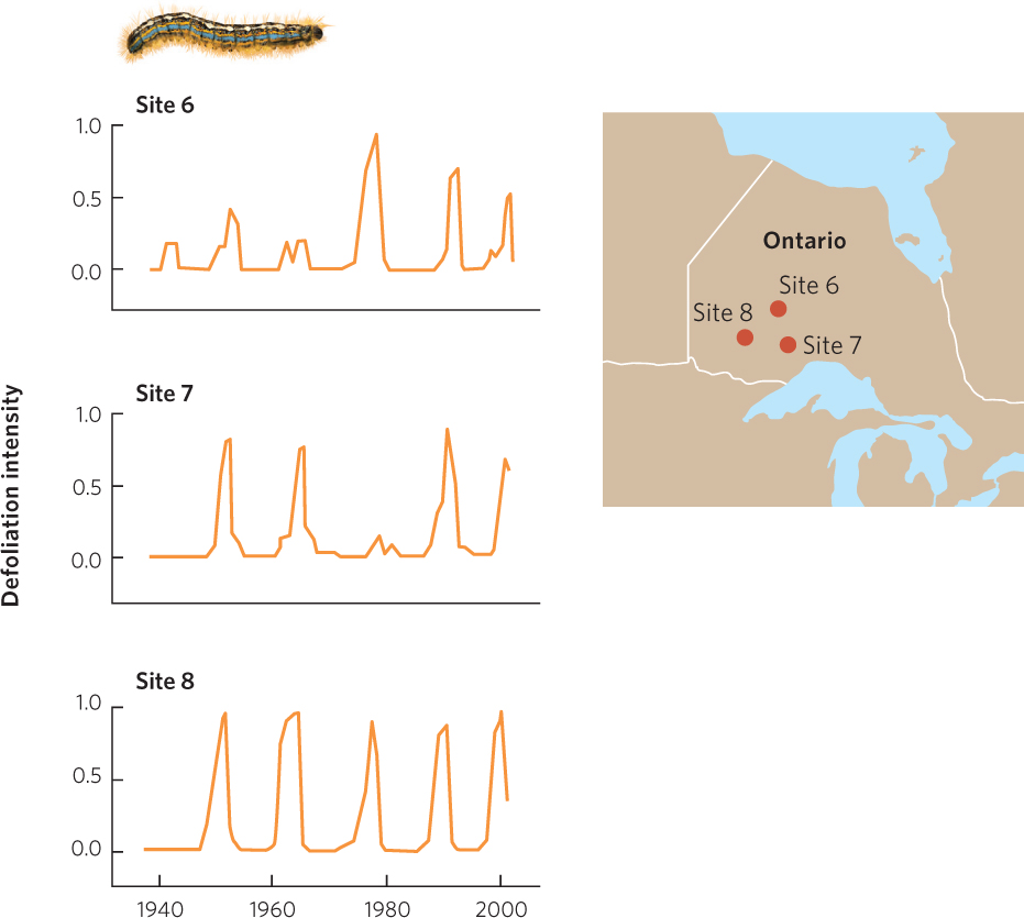
As we discussed in the previous chapter, the density of hosts can affect how easily parasites are transmitted from one host to another. An excellent example of this can be seen in the dynamic between the forest tent caterpillar (Malacosoma disstria)—a major herbivore of broadleaf trees in the United States and Canada— and a group of viruses that can infect and kill the caterpillar. The forest tent caterpillar can defoliate trees over thousands of square kilometers. In years of high caterpillar densities, they remove the majority of a tree’s leaves and tree growth is reduced up to 90 percent. In 2012, researchers in Canada reported that caterpillar populations had cycles that last 10 to 15 years and that these fluctuations were fairly synchronous across large geographic areas. In three different locations in the province of Ontario, the fluctuations in caterpillar populations exhibit the same pattern of growth and decline over time, as shown in Figure 15.13. Although the caterpillar is susceptible to predators and parasitoids, viruses have the greatest ability to reduce its abundance. When the tent caterpillar population is high, the virus comes into contact with new hosts more frequently and each caterpillar is more likely to get the virus. Under these conditions, large numbers of caterpillars die. As host population density decreases, it becomes harder for the viruses to find a new host and the prevalence of the disease declines. Since fewer caterpillars become infected and die, the caterpillar population starts to increase again.

Figure 15.13 Cyclic population fluctuations of forest tent caterpillars. At three sites in the province of Ontario, researchers quantified the population sizes of tent caterpillars by measuring the intensity of leaf removal on the trees. Over a 60-year period, the caterpillars exhibited large population fluctuations every 10 to 15 years. The rapidly growing populations ultimately succumb to an outbreak of infection by a virus and the populations quickly die back.

Data from B. J. Cooke et al., The dynamics of forest tent caterpillar outbreaks across east-central Canada, Ecography 35 (2012): 422–435.

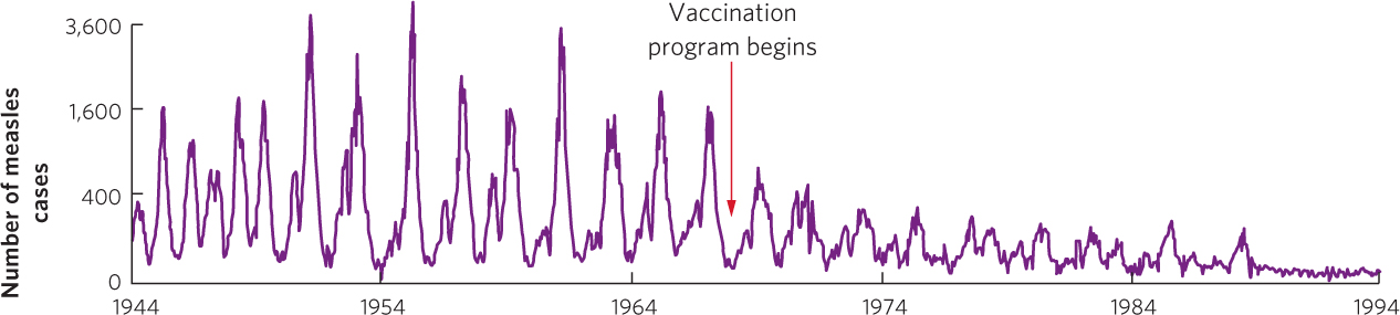
Fluctuations in parasite and host populations can also be caused by changes in the proportion of the host that has achieved immunity. When a host species possesses the ability to become immune to a parasite after an initial infection, continued infection in the population causes an increasing proportion of the population to develop immunity. When a high proportion of the population is no longer susceptible to the parasite, its spread is slowed. Measles, for example, is a highly contagious viral disease that stimulates lifelong immunity in humans. In unvaccinated populations, measles typically produces epidemics at 2-year intervals. Once most of the population is infected and develops immunity, the number of new measles cases declines sharply. As humans continue to reproduce, however, there are enough new children born without immunity to initiate another measles outbreak after 2 years. The number of measles cases in London, England, from 1944 to 1968—before vaccinations became available— shows a distinct pattern of 2-year cycles, as you can see in Figure 15.14. Once vaccinations became available and a higher proportion of susceptible individuals were immunized, the number of new cases dropped sharply and the fluctuations declined and eventually disappeared.

Figure 15.14 The cyclical occurrence of measles in a human population. Before vaccinations became available in 1968, the human population in London, England, experienced cycles of measles every 2 years. Once vaccination became available and the number of people getting vaccinated increased, the number of measles cases declined and the fluctuations no longer occurred.

Data from P. Rohani et al., Opposite patterns of synchrony in sympatric disease metapopulations, Science 286 (1999): 968–971.

Modeling Parasite and Host Populations

For pathogenic parasites, we can understand the dynamics of the parasite and the host using models that are similar to the Lotka-Volterra predator–prey model. However, the parasite–host model differs from the predator–prey model in two key ways. Parasites, unlike predators, do not always remove host individuals from a population, and hosts may develop immune responses that make some individuals resistant to the pathogen.

The simplest model of infectious disease transmission that incorporates immunity is the Susceptible-Infected-Resistant (S-I-R) model. In this model, all individuals begin as susceptible to the pathogen (S). Of those, some number becomes infected (I). Of the infected individuals, some number develops resistance via immunity (R). We can use this model to examine the conditions that favor an epidemic versus the conditions that cause a disease to decline. The proportions of S, I, and R individuals in a population are determined by rates of transmission of the disease and acquisition of immunity, as well as the birth of new, susceptible individuals.

In a population of hosts, the first individual to be infected by a pathogen is known as the primary case of the disease. Any individuals infected from this first individual are known as secondary cases. The rate at which the pathogen spreads through the population depends on two opposing factors. One factor is the rate of transmission between individuals (b), which includes both the rate of contact of susceptible individuals with an infectious individual and the probability of infection when there is contact. The other factor is the rate of recovery (g), which determines the period of time from when an individual is infected and can transmit the infection to when the individual’s immune system clears the infection and the individual becomes resistant to any future infections.

The rate of infection and the rate of recovery can be used to determine whether an infectious disease will spread through a population. A disease will spread whenever the number of newly infected individuals is greater than the number of recovered individuals. To determine the number of newly infected individuals, we need to know the probability that an infected individual and a susceptible individual will come into contact with each other. If we assume that individuals in the population move around randomly, the probability of contact is the product of their proportions in the population:

Once infected and susceptible individuals come into contact, we also have to consider the rate of infection between them (g):

Next we have to determine how many individuals are recovering from the infection. We can do this by knowing the proportion of infected individuals (I) and the rate of recovery from an infection (b):

Now we can determine whether an infection will spread through a population. To do this, we need to calculate the reproductive ratio of the infection (R₀), which is the number of secondary cases produced by a primary case during its period of infectiousness.

The reproductive ratio of the infection is the ratio of new infections to recoveries:

If R₀ > 1, the infection will continue to spread through the population and an epidemic will occur. This happens because each infected individual infects more than one other individual before it recovers from the disease and becomes resistant. When R₀ < 1, the infection fails to take hold in the host population. This happens because each infected individual fails to infect another individual, on average, before it recovers and becomes resistant.

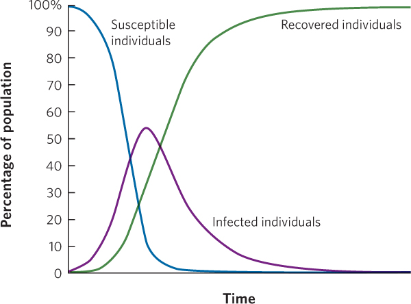
Figure 15.15 illustrates the dynamics of a typical disease. Imagine that we start with a population that is composed entirely of uninfected individuals. When an infectious disease arrives, there is initially a rapid increase in the number of infected individuals but, over time, infected individuals subsequently recover and become resistant (R). At this point, the number of susceptible individuals (S) decreases, so the value of R₀ decreases. When R₀ declines to < 1, the growing epidemic can no longer sustain itself. As a result, the number of infected individuals achieves a peak in abundance and then declines.

Figure 15.15 The dynamics of an infection over time. In the basic S-I-R model, all individuals in a population are initially susceptible. When the infection is introduced at the beginning of the time period, there is an initial rapid growth in the number of infected individuals. As some infected individuals recover and become resistant, there are fewer susceptible individuals left to infect, so the number of infected individuals declines.

With this understanding of how R₀ affects the spread of diseases, we can now look at the R₀ values for different diseases that are caused by parasites. HIV is transmitted through rather limited mechanisms including direct sexual contact, blood transfusion, or perinatal transmission from mother to offspring. HIV has a relatively low range of R₀ values, from 2 to 5. Typical values for R₀ in childhood diseases of humans—measles, chicken pox, and mumps, among others—range from 5 to 18 at the time a population is initially infected. At the extreme, malaria, which is transmitted by mosquitoes, has an R₀ value greater than 100 in crowded human populations. This high value occurs because mosquitoes are excellent vectors for transmitting the parasite and infected people remain infectious for long periods of time.

Assumptions of the S-I-R Model

The basic S-I-R model has several important assumptions. For example, it assumes there are no births of new susceptible individuals and that individuals retain any resistance they develop. In such a model, the result is an epidemic that runs its course until all individuals in the population have become resistant or there are too few susceptible individuals remaining to sustain the spread of the disease. Some pathogens, such as influenza viruses, fit these assumptions. The basic model also explains why vaccinations slow or stop the spread of diseases such as influenza; by vaccinating individuals, we reduce the size of the susceptible population (S), which reduces the value of R₀. This makes it harder for an epidemic to sustain itself.

Other factors can be added to the model, including births of susceptible infants, lag times between when an individual is infected and becomes infectious to others, host mortality, host population dynamics, and transmission of disease from parent to offspring. These additional factors can have substantial effects on the predictions of the model. For example, the birth of new susceptible individuals can cause cyclic fluctuations in the model, as we observed in the case of the measles data from London (Figure 15.14).

If a pathogen can kill the host, the pathogen should increase in abundance until the hosts begin to die. As the host population declines, the pathogen population will subsequently decline and as the pathogen population declines, the host population should subsequently recover. This is analogous to the predator–prey cycles we discussed in Chapter 14. However, some pathogens do not follow these dynamics because they do not attack a single host species. For instance, the chytrid fungus that we discussed earlier in this chapter infects dozens of species of amphibians. A host species can decline all the way to extinction, yet the fungus does not decline in abundance because it can infect other species of amphibians. Some of these newly infected species will become ill and die while others never develop the disease and serve as reservoirs for the disease. When a pathogen is not restricted to a single host species, it has the ability to persist and spread even after it causes one of its hosts to go extinct.