Evolution can occur through random processes or through selection
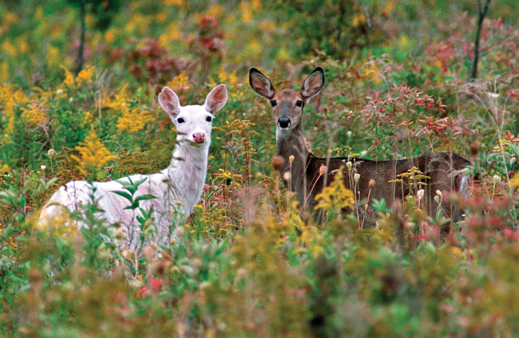
In western New York State there is a herd of white-tailed deer that looks very different from most white-tailed deer. Many of the deer living on the 4,300-ha Seneca Army Depot do not have typical reddish brown coats. Rather, their coats are white (Figure 7.4). The white coat phenotype is due to a rare mutation that occurs throughout the range of white-tailed deer. Because a white coat can frequently make a deer more visible to predators, it does not provide any fitness benefits and we would not expect it to persist. So why is there a high frequency of white deer on the Seneca Army Depot? It turns out that when the army depot was built in 1941, the 4,300-ha area was fenced and several dozen deer were trapped inside. A few years later, 2 white deer were observed. Given that white deer were such an unusual sight, authorities at the depot banned hunters from killing the deer with the white phenotype. Over time, the deer population grew larger and the white phenotype became more frequent. Today, of the nearly 800 deer living on the property, about 200 are white.
166
The story of the white deer demonstrates how evolution often happens through multiple processes. Random events, such as mutations, may confer no fitness advantage when they first appear. Such is the case for most deer populations in which the white mutation occasionally arises. However, if selection for the mutant phenotype begins to occur, as happened at the Seneca Army Depot with reduced hunting pressure, the mutant can become more frequent in the population.
Evolution Through Random Processes
As we saw with the mutation that causes white deer, random processes can facilitate evolutionary change in a population. In addition to mutation, random processes include genetic drift, bottleneck effects, and founder effects.
Mutation
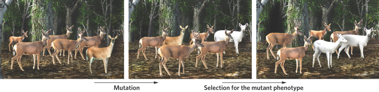
We have seen that mutation is one of the two primary ways that genetic variation arises in a population. Because genes often code for functions that are vital to performance and fitness, mutations that negatively impact these functions are not favored by selection. However, a small fraction of mutations can be beneficial. For example, Figure 7.5 illustrates what happened in the deer herd of the Seneca Army Depot. In a herd of deer, a mutation for the white coat appeared, which added genetic variation to the population. After the mutation appeared and became protected, the frequency of white deer increased.
Mutation rates vary a great deal in different groups of organisms, but among genes that are expressed and can be observed as altered phenotypes mutation rates range from 1 in 100 to 1 in 1,000,000 per gene per generation. The more genes that a species carries, the higher the probability that at least one gene will experience a mutation. Similarly, the larger the size of the population, the higher the probability that an individual in the population will carry a mutation.
Genetic Drift
Genetic drift A process that occurs when genetic variation is lost because of random variation in mating, mortality, fecundity, and inheritance.
Genetic drift, another random process, occurs when genetic variation is lost because of random variation in mating, mortality, fecundity, or inheritance. Genetic drift is more common in small populations because random events can have a disproportionately large effect on the frequencies of genes in the population. But how does one determine whether an evolved phenotype is the outcome of drift versus some other process, such as natural selection? Research on the Mexican cavefish (Astyanax mexicanus) provides an answer.
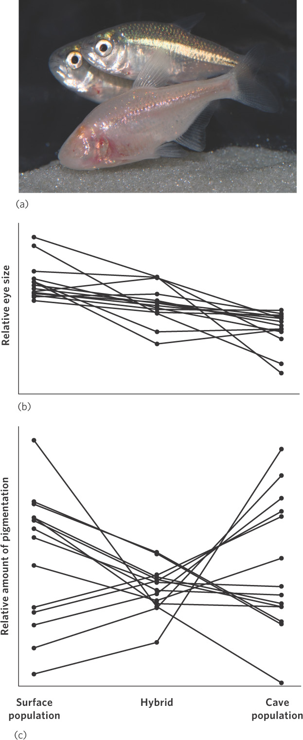
The Mexican cavefish is a species composed of some populations that live in cave streams and other populations that live in surface streams. Although the populations can interbreed, they look quite different. As is the case with many cave-adapted animals, the cave populations have very reduced eyes and reduced pigmentation (Figure 7.6a). However, populations living in surface streams have normal eyes and dark pigmentation. To determine whether these changes were due to natural selection or to genetic drift, researchers raised individuals from the cave population, individuals from the surface population, and hybrid offspring made by interbreeding the cave and surface populations. The researchers then examined regions of the fish DNA that coded for eye size and pigmentation, which could contain one or more genes. In 2007, they reported that the 12 regions of DNA that coded for large eyes in the surface population all coded for small eyes in the cave population. The results are shown in Figure 7.6b. This suggests that natural selection favored all of the eye genes to evolve in a similar direction to produce smaller eyes. In contrast, when they examined the 13 regions of DNA that coded for pigmentation, they found that 5 of the regions coded for increased pigmentation in the cave populations and 8 of the regions coded for decreased pigmentation, as shown in Figure 7.6c. The lack of a consistent pattern among the 13 regions of DNA suggests that natural selection was not involved. Instead, the differences in pigmentation in the cavefish populations were likely produced by genetic drift. Given that small populations tend to experience more genetic drift than large populations, it may be the case that the cave population was initially very small.
167
Bottleneck Effects
Bottleneck effect A reduction of genetic diversity in a population due to a large reduction in population size.
A reduction in genetic variation can also occur because of a severe reduction in population size, known as the bottleneck effect. When a population experiences a large reduction in the number of individuals, the survivors carry only a fraction of the genetic diversity that was present in the original, larger population. Moreover, after being reduced to a small population by the bottleneck effect, the small population can then experience genetic drift. Population reductions can happen from natural causes, for example a drought that reduces the abundance of food, or anthropogenic causes, such as loss of habitat due to the construction of homes or factories.
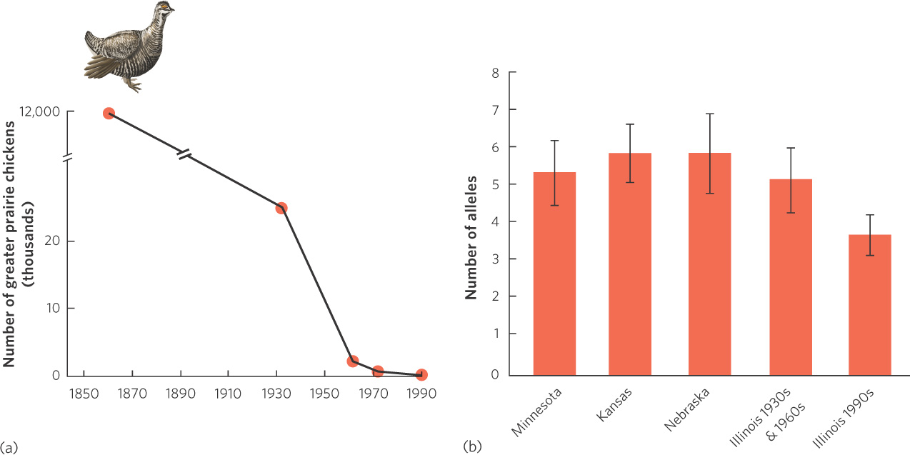
One example of a bottleneck effect is the greater prairie chicken (Tympanuchus cupido), which is a grassland bird that historically lived throughout much of the middle United States, including Minnesota, Kansas, Nebraska, and Illinois. While prairie chickens have remained abundant in many states, the population in Illinois declined from approximately 12 million in 1860 to only 72 birds by 1990, as illustrated in Figure 7.7a. To determine whether this dramatic decline in population size was associated with a decline in genetic diversity, researchers collected DNA samples from museum specimens of prairie chickens from the 1930s, when the population was 25,000, and from the 1960s, when the population was 2,000. They defined this time period from the 1930s to the 1960s as “pre-bottleneck.” They also compared the genetic diversity of the Illinois birds before and after the bottleneck to the genetic diversity in the present-day populations of prairie chickens in Minnesota, Kansas, and Nebraska. In all cases, they examined the number of alleles that a population contained for each of six different genes. As shown in Figure 7.7b, the large populations of the neighboring states and the large historic population in Illinois all contained a high number of alleles. The current population in Illinois, however, has a lower number of alleles, which reflects the genetic bottleneck effect. The state of Illinois has since purchased more prairie habitat and introduced hundreds of prairie chickens from neighboring states to help bolster the Illinois population and increase its genetic diversity.
168
The bottleneck effect is of particular interest because the subsequent reduction in genetic diversity may prevent the population from adapting to future environmental changes. This is especially true for organisms that face deadly pathogens. An inability to evolve against new strains of a pathogen could lead to the extinction of the host organism. For example, the African cheetah (Acinonyx jubatus) experienced a population bottleneck approximately 10,000 years ago. Although the cause of that bottleneck is unknown, the current population contains very little genetic variation. This low genetic variation makes cheetahs more vulnerable to pathogens, including a deadly pathogen that causes the disorder known as AA amyloidosis and kills up to 70 percent of cheetahs held in captivity.
Founder Effects
Founder effect When a small number of individuals leave a large population to colonize a new area and bring with them only a small amount of genetic variation.
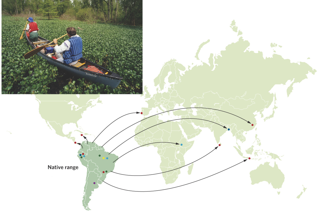
The founder effect occurs when a small number of individuals leave a large population to colonize a new area and bring with them only a small amount of genetic variation. Following the founding by this small population, genetic drift can cause additional reductions in genetic variation. The genetic variation remains low until enough time has passed to accumulate new mutations. The water hyacinth (Eichhornia crassipes), which has been introduced by humans to many parts of the world, provides an example of the founder effect. Water hyacinth is an aquatic plant that is native to South America. During the past 150 years, the plant has been either accidentally or intentionally introduced to many other parts of the world. Once introduced, it grows and spreads quite rapidly, dominating shallow-water areas and displacing native plants. Today, water hyacinth has become one of the most invasive plants in the world.
169
Because most water hyacinth introductions are thought to have happened with few individuals, researchers wondered if the plant would show indications of founder effects in those parts of the world where it was not native. They sampled 1,140 plants from around the world and determined their genotypes. In 2010, they reported a single widespread genotype occurred in 71 percent of the sampled plants and this genotype dominated 75 percent of all populations that were outside the plant’s native range, as shown in Figure 7.8. Moreover, 80 percent of all populations outside the native range were composed of a single genotype, whereas populations in the native range of South America had up to five different genotypes. This pattern suggests that there were few founders in the invaded regions of the world and that they contained a small proportion of the genetic diversity of native populations in South America.
Evolution Through Selection
Selection The process by which certain phenotypes are favored to survive and reproduce over other phenotypes.
The nonrandom process of selection also plays a substantial role in evolution. Selection is the process by which certain phenotypes are favored to survive and reproduce over other phenotypes. As we saw in the story of the medium ground finches at the beginning of this chapter, selection is a powerful force that can change the phenotypes (and therefore the gene frequencies) of a population in a relatively short period of time. Depending on how the environment varies over time and space, selection can influence the distribution of traits in a population in three ways: stabilizing selection, directional selection, and disruptive selection.
Stabilizing Selection
Stabilizing selection When individuals with intermediate phenotypes have higher survival and reproductive success than those with extreme phenotypes.
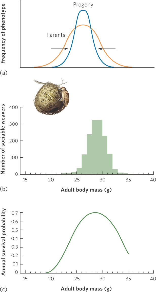
When individuals with intermediate phenotypes have higher survival and reproductive success than those with extreme phenotypes, we call it stabilizing selection. As shown in Figure 7.9a, stabilizing selection begins with a relatively wide distribution of phenotypes, as illustrated by the orange line. After stabilizing selects for parents who possess intermediate phenotypes, their progeny have a more narrow distribution of phenotypes, as illustrated by the blue line. In doing so, it performs genetic housekeeping for a population, sweeping away harmful genetic variation. An example of stabilizing selection can be seen in selection for body mass in a species of bird from South Africa called the sociable weaver (Philetairus socius). Over an 8-year period, researchers marked nearly 1,000 adult birds and examined how a bird’s mass was related to its subsequent survival. As you can see in Figure 7.9b, the mass of the adults in the study follows a normal distribution with a mean of approximately 29 g. The researchers then asked how well birds of different mass survive. When mass was graphed against survival, as shown in Figure 7.9c, they found that the smallest and largest birds survived poorly, whereas birds of intermediate mass survived the best. That is, selection favored the intermediate phenotype. When the environment of a population is relatively unchanging, stabilizing selection is the dominant type of selection. Because the average phenotype does not change, little evolutionary change takes place.
170
Directional Selection
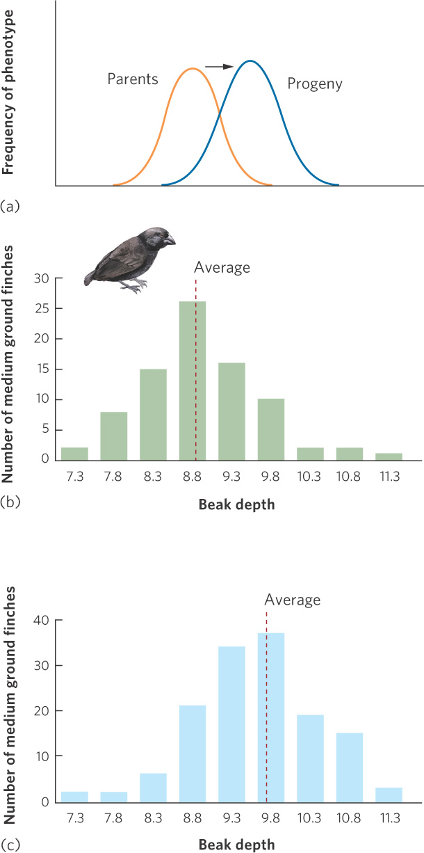
At the beginning of this chapter, we saw that beak size of the medium ground finch evolved to be larger during a drought when only the large seeds were available. This is an example of directional selection, which occurs when an extreme phenotype experiences higher fitness than the average phenotype of the population, as shown in Figure 7.10a. In the medium ground finch, for example, Peter and Rosemary Grant quantified the distribution of beak sizes in offspring hatched in 1976, which was just prior to a drought. As you can see in Figure 7.10b, the beak sizes of these offspring followed a normal distribution with a mean beak depth of 8.9 mm. When the drought came, although all seeds became less abundant, there were proportionately more large seeds remaining. The large seeds are harder to crack, so birds with deeper beaks were better able to feed on hard seeds and they had better survival. Because beak depth is a heritable trait, the offspring that were hatched in 1978 had deeper beaks, as shown in Figure 7.10c.
Directional selection When individuals with an extreme phenotype experience higher fitness than the average phenotype of the population.
Disruptive Selection
Disruptive selection When individuals with either extreme phenotype experience higher fitness than individuals with an intermediate phenotype.
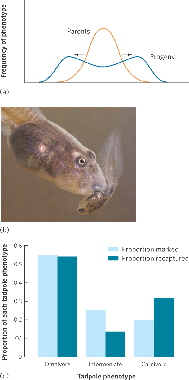
Under some circumstances, we see another type of selection known as disruptive selection. In disruptive selection, individuals with extreme phenotypes at either end of the distribution can have higher fitness than individuals with intermediate phenotypes. Disruptive selection is illustrated in Figure 7.11a. For example, tadpoles of the Mexican spadefoot toad (Spea multiplicata) can express a range of possible phenotypes that are related to what they eat. At one extreme is the omnivorous phenotype that has small jaw muscles, numerous little teeth, and a long intestine that makes it well suited for feeding on detritus. At the other extreme is the carnivorous phenotype that has large jaw muscles, a notched mouthpart, and a short intestine that makes it well suited for feeding on freshwater shrimp and cannibalizing conspecifics. Intermediate phenotypes are not well suited to feed on either of the two food types. To test whether the tadpoles experienced disruptive selection, researchers collected more than 500 tadpoles from a desert pond, marked them to indicate their phenotype, and then returned them back to their pond. They sampled the pond again 8 days later to determine the survival of the three phenotypes. As you can see in Figure 7.11b, the omnivorous and carnivorous phenotypes survived relatively well, but the intermediate phenotypes—which had intermediate jaw muscles, tooth number, and intestine length—survived poorly. Because disruptive selection removes the intermediate phenotypes, it increases genetic and phenotypic variation within a population. In doing so, it creates a distribution of phenotypes with peaks toward both ends of the original distribution.
171
172
ANALYZING ECOLOGY
Strength of Selection, Heritability, and Response to Selection
Researches often wish to know exactly how much selection will move the mean phenotype in a population. For example, if a plant breeder selects for larger tomato plants, she might want to know how much larger the next generation will be. Similarly, a government agency that regulates fishing might want to know if harvesting only the largest individuals might cause the population to evolve to be smaller in the next generation.
Let’s consider the case of directional selection in which one end of the phenotypic distribution is favored. If there is selection for more extreme phenotypes and the phenotype has a genetic basis, directional selection will cause the mean phenotype to change. Can we determine exactly how much the mean phenotype will change in the next generation? To answer this question we need to know both the strength of selection of the phenotype and the heritability of the phenotype.
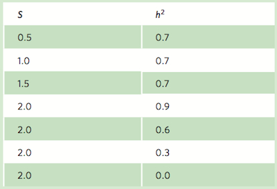
Strength of selection The difference between the mean of the phenotypic distribution before selection and the mean after selection, measured in units of standard deviations.
The strength of selection is the difference between the mean of the phenotypic distribution before selection and the mean after selection, measured in units of standard deviations (see Chapter 2). For example, imagine that we wanted to select for larger tomatoes. The phenotype (tomato mass) follows a normal distribution with a mean of 100 g and a standard deviation of 10 g. Now imagine that we select the upper end of the distribution and use these individuals to breed the next generation of tomatoes. If this selected group has a mean of 115 g, our selected group has a mean that is 1.5 standard deviations away from the mean of the entire population. Thus, the strength of selection is 1.5.
Heritability The proportion of the total phenotypic variation that is caused by genetic variation.
We also know that phenotypes are the products of genes and the environment. Since only genetic material can be passed down to the next generation, if we wish to know how much the mean phenotype will change, we have to determine what proportion of the total phenotypic variation is caused by genes. This proportion is called the heritability and it can range between 0 and 1. If all of the phenotypic variation that we see in a normal distribution is due to the environment, the heritability is 0. If all of the phenotypic variation is due to genetic variation, the heritability is 1. By convention, the symbol for heritability is h2. (This notation may be confusing because nothing is being squared.)
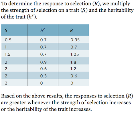
Using the concepts of strength of selection and heritability, we can build an equation that describes how much a population will respond to selection in the next generation. Because a population’s response to selection is a function of the strength of selection and the heritability of the phenotype
R = S × h2
where R is the response to selection, S is the strength of selection, and h2 is the heritability.
Using our tomato example, we can calculate how much larger the tomatoes should be in the next generation. If we select parents that are 1.5 standard deviations above the population mean and if the heritability is 0.33, then
R = 1.5 × 0.33 = 0.5
which means that the mean phenotype of the next generation of tomatoes will be 0.5 standard deviations—or 5 g—greater than that of the parent’s generation.
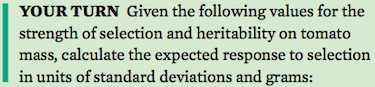
Based on your calculations, how is the response to selection affected by the strength of selection and heritability?
173