Life history traits are shaped by trade-offs
If we consider the many types of life history traits, it would seem that an organism could have very high fitness if it could grow fast, achieve sexual maturity at an early age, reproduce at a high rate, and have a long life span. However, no organism possesses the best of all such life history traits, which highlights the fact that organisms face trade-offs. When one life history trait is favored, it often prevents the adoption of another advantageous life history trait. In some cases, there are physical constraints, such as the size of a mammal’s uterus, which places a limit on the total volume of offspring that can be produced at one time. Thus, a female can produce several small offspring, or a few large offspring, but not many large offspring. In other cases, the trade-off reflects the genetic makeup of the organism. Because some genes have multiple effects, selection that favors genes for one life history trait can cause other life history traits to change. For instance, in the mouse-ear cress (Arabidopsis thaliana), artificial selection for earlier flowering also causes reduced seed production. In still other cases, the trade-offs are the result of the allocation of a finite amount of time, energy, or nutrients. Given the large number of life history traits, there are many potential trade-offs. In this section, we will discuss the principle of allocation and highlight some of the most common trade-offs that have been observed.
The Principle of Allocation
Principle of allocation The observation that when resources are devoted to one body structure, physiological function, or behavior, they cannot be allotted to another.
Organisms often have limited time, energy, and nutrients at their disposal. According to the principle of allocation, when these resources are devoted to one body structure, physiological function, or behavior, they cannot be allotted to another. As a result, natural selection will favor those individuals that allocate their resources in a way that achieves maximum fitness.
Selection on life history traits can be complex because when one trait is altered, it often influences several components of survival and reproduction. As a result, the evolution of a particular life history trait can be understood only by considering the entire set of consequences. For example, an increase in the number of seeds an oak tree produces may contribute to higher fitness. However, if a higher number of seeds is achieved by making each seed smaller, and if smaller seeds experience lower survival, then producing more seeds could negatively affect the tree’s overall fitness. In this case, to achieve an outcome that maximizes overall fitness, evolution should favor a strategy that balances the trade-off between seed number and seed survival.
From an evolutionary point of view, individuals exist to produce as many successful progeny as possible. Doing so, however, involves many allocation problems, including the timing of sexual maturity, the number of offspring to have at any one time, and the amount of parental care to bestow upon the offspring. An optimized life history is one that resolves conflicts between the competing demands of survival and reproduction to the best advantage of the individual in terms of its fitness. Although it is widely believed that trade-offs constrain life histories, demonstrating such trade-offs has proved difficult. In some cases, trade-offs can only be exposed by using experimental manipulations.
Offspring Number Versus Offspring Size
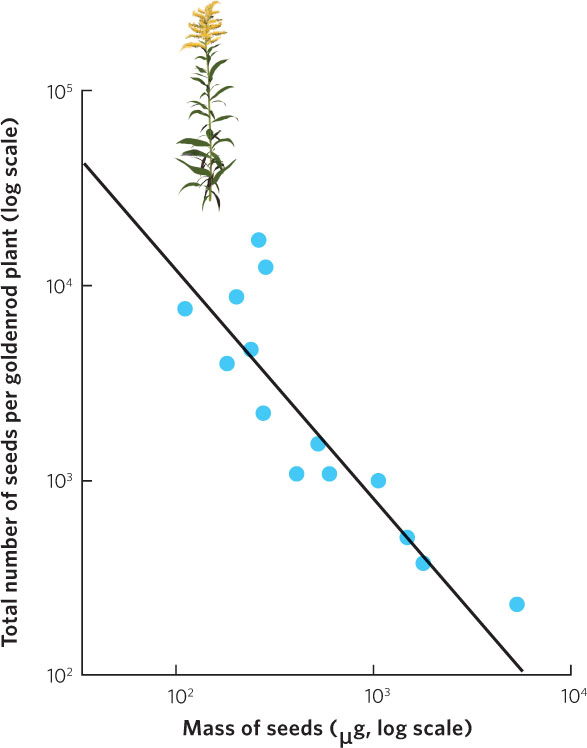
Most organisms face a trade-off between the number of offspring they can produce and the size of those offspring in a single reproductive event. As we noted for mammals, the number of offspring in any given pregnancy can only increase if the size of each individual offspring decreases. The trade-off between offspring number and offspring size for a given reproductive event can also be limited by energy and nutrients. An example of this can be seen in Figure 8.3, which illustrates the relationship between seed size and seed number in plants of the goldenrod genus (Solidago). Across populations and species, there is a negative correlation, demonstrating that goldenrod plants that produce more seeds also produce smaller seeds. However, although the trade-off between offspring number and offspring size can be seen in a number of species, the expected trade-off is often not observed. In many cases, while the number of offspring can be quite variable among individuals, the size of offspring can be relatively constant. This suggests that selection often favors a uniform, perhaps even optimal, offspring size and that an individual able to acquire additional energy can only use it to make greater numbers of offspring.
190
ANALYZING ECOLOGY
Coefficients of Determination
When ecologists want to look for life history trade-offs, they commonly plot one life history variable against another life history variable and look for a negative relationship. We saw an example of this in the case of the goldenrod seeds; the researchers used a regression to demonstrate a trade-off between seed number and seed size. As we saw in Chapter 5, a regression is a mathematical description of the relationship between two variables. For example, data points that tend to follow a straight line might be best described by using a linear regression described by the following equation:
Coefficient of determination (R2) An index that tells us how well data fit to a line.
Y = mX + b
where X and Y are the measured variables, m is the slope—which is negative in the case of the goldenrod example—and b is the intercept.
Although this equation tells us how one variable is associated with another variable, it does not tell us how strongly the two variables are related. For example, it would be valuable to know if the data points fit closely along the line or if the data points are highly variable around the line. We can answer this question using a statistic known as the coefficient of determination. The coefficient of determination, which is abbreviated as R2, is an index that tells us how well data fit to a line. Values can range from 0 to 1, with 0 indicating a very poor fit of the data and 1 indicating a perfect fit of the data. In terms of life history trade-offs, higher R2 values indicate that a variation in one life history trait explains a large amount of the variation in the other life history trait.
Consider the following set of hypothetical data for plant seeds that all have the same linear relationship between seed mass and seed number, as given in the equation:
Seed mass = (−4 × Seed number) + 24
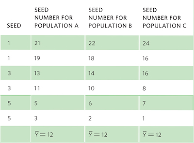
For each set of data, we can graph the relationships and include the regression line, as shown in the graphs below.
To calculate R2, we need to first calculate the mean Y value, which for all populations is a seed number of 12. We also need to determine the expected seed numbers if the data were to fall perfectly along the line. Using the line equation and the above data for seed mass, the six expected seed numbers are 20, 20, 12, 12, 4, and 4.
Next, we need to calculate the total sums of squares, which is the sum of the squared differences between each observed seed number (yi) and the mean seed number  :
:

Next we calculate the error sums of squares, which is the sum of the squared differences between each expected seed number (fi) and the observed seed number (yi):

Finally, we can calculate the value of R2 as follows:
For population A, we can calculate the value of R2 as follows:
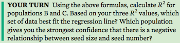
For Population A:
For Population B:
For Population C:

Because of the higher coefficient of determination, Population A provides the strongest confidence that thereis a negative relationship between seed size and seed number.
191
Offspring Number Versus Parental Care
The number of offspring produced in a single reproductive event can also cause a trade-off with the amount of parental care that can be provided. As the number of offspring increases, the efforts of the parents to provide food and protection will increasingly be spread thin. Presumably, there is an optimal number of offspring for parents to produce.
In a classic study of life history evolution, David Lack of Oxford University considered the number of offspring produced by songbirds. Lack observed that songbirds breeding in the tropics lay fewer eggs at a time—an average of 2 or 3 per nest—than songbirds breeding at higher latitudes, which, depending on the species, typically lay 4 to 10 eggs. In 1947, he proposed that these different reproductive strategies evolved in response to differences between tropical and temperate environments. Lack recognized that birds could improve their overall reproductive success by increasing the number of eggs, as long as a larger number of offspring did not cause a decrease in offspring survival. He hypothesized that the ability of parents to gather food for their young was limited and, if they could not provide enough, the offspring would be undernourished and therefore less likely to survive. We should therefore expect that parents produce the number of offspring that they can successfully feed. One difference between the tropics and higher latitudes is the number of daylight hours. Lack noted that parents at higher latitudes had more hours to gather food to feed their young. Therefore, assuming that the rate of food gathering is similar at low and high latitudes, he hypothesized that birds breeding at high latitudes could rear more offspring than birds breeding in the low latitudes of the tropics.
192
Lack made three important points. First, he stated that life history traits, such as the number of eggs laid in a nest, not only contribute to reproductive success but also influence evolutionary fitness. Second, he demonstrated that life histories vary consistently with respect to factors in the environment, such as the number of daylight hours available for gathering food for their young. This observation suggested that life history traits are molded by natural selection. Third, he hypothesized that the number of offspring parents can successfully rear is limited by food supply. To test this idea, one could add eggs to nests to create unnaturally high numbers of hatchlings. According to Lack’s hypothesis, parents should not be able to rear larger broods of chicks because they cannot gather the additional food that is required.
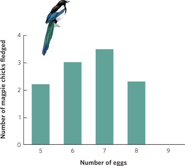
Such experiments have been conducted many times during the last several decades and Lack’s hypothesis has commonly been supported. For example, the European magpie (Pica pica) typically lays seven eggs in its nest. To determine whether this is the most fit strategy for the magpie, researchers manipulated the number of eggs in magpie nests by removing one or two eggs from several nests and adding these eggs to other nests. To control for their disturbance of the nests, they also switched eggs between nests without changing their number. The researchers then waited to see how many chicks could be raised to the fledgling stage, when the offspring can leave the nest. As shown in Figure 8.4, magpies that had fewer than seven eggs or more than seven eggs ended up producing fewer fledgling birds. Nests that had eggs removed produced fewer fledglings because they started with fewer offspring. In contrast, nests with eggs added produced fewer total fledglings because the chicks had to share the food with more siblings. This competition with siblings caused the chicks to grow more slowly and experience higher mortality rates because the parents were unable to feed so many offspring. As Lack predicted, the number of eggs the magpie produces maximizes the number of offspring it can successfully raise.
Fecundity and Parental Care Versus Parental Survival
We saw how adding eggs to the nests of birds increased competition among the young for food that the parents brought. Consequently, parents with broods of intermediate size have the greatest fitness. Sometimes, however, having more mouths to feed stimulates parents to hunt harder for food for their chicks. In this case, an artificially enlarged brood might result in higher reproductive success in the short term. However, the additional parental effort can impose a cost on the parents that affects their subsequent fitness.
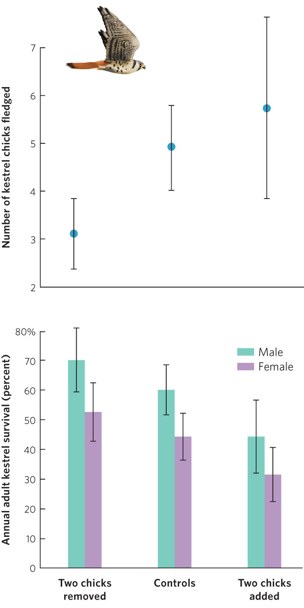
European kestrels (Falco tinnunculus) provide an example of the trade-off between fecundity and parental survival. Kestrels are small falcons that feed on voles and shrews caught in open fields. While foraging requires a high rate of energy expenditure, the small mammals are so abundant that kestrel pairs normally can catch enough prey to feed their brood in a few hours each day. Kestrels lay an average of five eggs per brood. In one study, when chicks were about a week old, broods in a sample of nests were subjected to one of three manipulations: investigators removed two chicks from a nest, switched chicks between nests without changing their number, or added two chicks to a nest. Investigators expected that parents of the artificially reduced and enlarged clutches would alter the amount of energy they expended looking for food for the chicks.
While parents with fewer eggs ultimately had fewer chicks fledge than the control group, parents with additional eggs had more chicks fledge, as shown in Figure 8.5. However, in spite of the increased hunting efforts of their parents, chicks in the enlarged broods were somewhat undernourished and only 81 percent survived to fledge, compared with 98 percent survival in control nests and in nests with eggs removed. Consequently, the extra hunting effort to feed the additional two chicks only netted the parents an extra 0.8 chick, and this gain may have been diminished by the later deaths of some of the underweight fledglings. Moreover, the increased hunting efforts caused lower survival of these adults into the next breeding season. This means that increasing the number of offspring provides diminishing benefits to the parents in terms of the number of offspring that survive. Simultaneously, it causes greater adult mortality because parents must spend more energy securing food. At some point, the gains made by increasing current reproduction, which requires a large increase in parental care, are offset by the increased adult mortality, which reduces the chance of future reproduction.
193
Growth Versus Age of Sexual Maturity and Life Span
Determinate growth A growth pattern in which an individual does not grow any more once it initiates reproduction.
Indeterminate growth A growth pattern in which an individual continues to grow after it initiates reproduction.
Organisms also commonly face a trade-off between putting their energy into growth or putting their energy into reproduction. In most species of birds and mammals, females grow to a particular size before they begin to reproduce. But once they initiate reproduction, females do not grow anymore—a phenomenon known as determinate growth. In contrast, many plants and invertebrates, as well as many fishes, reptiles, and amphibians, do not have a characteristic adult size. Rather, they continue to grow after initiating reproduction, a phenomenon known as indeterminate growth. Typically, indeterminate growth occurs at a decreasing rate over time.
Whether a species has determinate or indeterminate growth, the key feature shaping the trade-off between growth and reproduction is that larger females commonly produce more offspring. Because offspring production and growth draw on the same resources of assimilated energy and nutrients, increased fecundity during one year occurs at the cost of further growth that year. Moreover, for indeterminate growers, the reduced growth in one year can cause reduced fecundity in subsequent years. An organism with a long life expectancy should favor growth over fecundity during the early years of its life. In contrast, organisms with a short life expectancy should allocate their resources to producing eggs early in life rather than delaying reproduction and growing more. These predictions can be tested by examining the relationships among these life history traits across many different species and by conducting manipulative experiments on species in nature.
Comparisons Across Species
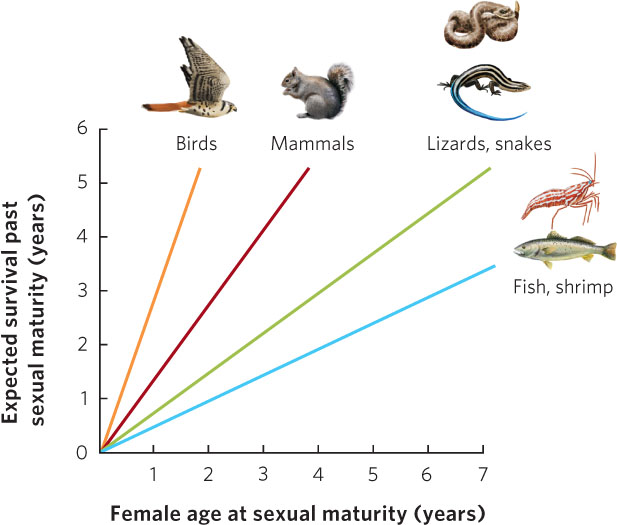
When we look across many different species, we see that long-lived organisms typically begin to reproduce later in life than short-lived ones. Why is this the case? If an organism has a long life span and if delaying maturity allows an organism to grow larger and produce more offspring per year once reproduction begins, natural selection will favor delayed age of maturity in these organisms. An analysis of hundreds of populations and species of animals illustrates this relationship. As you can see in Figure 8.6, as the age of sexual maturity increases, there is an associated increase in the number of years that an animal will survive after reaching sexual maturity. Moreover, different taxonomic groups fall along different regression lines. For species that are expected to live 2 years after sexual maturity, birds and mammals have the shortest times to sexual maturity whereas reptiles, fish, and shrimp have the longest times. This reflects the fact that endothermic animals can grow more rapidly than ectothermic animals. Among species with an age of maturity of 1 year, birds have the longest expected life spans after sexual maturity. This reflects the generally lower predation risk for birds due to their ability to fly.
194
Manipulative Experiments
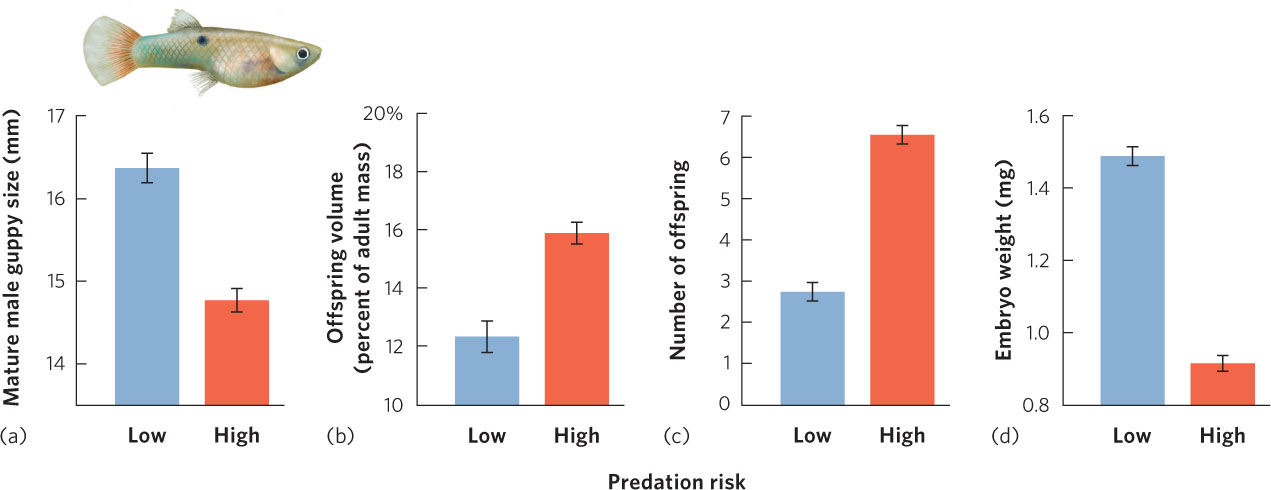
Another way to examine the trade-offs of growth, age of maturity, and life span is by conducting a manipulative experiment. The Trinidadian guppy (Poecilia reticulata), for instance, lives in the streams of Trinidad, a large island in the southern Caribbean Sea. In the lower reaches of these streams, the guppies live with a number of predatory fish species including the pike cichlid (Crenocichla alta), which preys on adult guppies, and the smaller killifish (Rivulus hartii), which preys primarily on juvenile guppies. Because of this predation, these guppies have short life expectancies. However, at higher elevations, where guppies have been able to ascend numerous small waterfalls, they live in a relatively predator-free environment and have longer life expectancies. Figure 8.7 shows the life history traits of guppy populations. In populations that face high predation risk and short life spans, males mature at smaller sizes. Females allocate more of their body mass to reproduction, they produce more offspring, and these offspring are smaller. As predicted, researchers found the opposite to be true for populations in the predator-free sections of the streams above the waterfalls: males matured at larger sizes and females allocated less of their body mass to reproduction and produced fewer, larger offspring.
Researchers then conducted a manipulative experiment to test the hypothesis that increased mortality from predation was actually the cause of the altered life history strategies of the local guppy populations. They transplanted predators from the lower reaches of the streams to the areas above the waterfalls where predators did not historically exist. Within a few generations, the life histories of the populations above the waterfalls came to resemble those of the populations in the lower reaches of the stream. This finding not only confirmed the basic ideas about the optimization of life history patterns, but also demonstrated the strength of predation as a selective force in evolution.
195