7.3 Populations display various patterns of growth.
Researchers involved in species’ restoration projects observe factors such as distribution, genetic diversity, initial population size, and density as well as prey availability and habitat structure, and evaluate how they influenced the size and dynamics of a vulnerable or reintroduced population. In order to predict population dynamics, scientists use some simple mathematical models that describe population growth over time. The annual population growth rate is determined by birth rate (the number of births per 1000 individuals per year) minus the population death rate (number of deaths per 1000 individuals per year), or by taking a simple census of population size at two time points. Between 2009 and 2010, the Yellowstone wolf population went from 320 to 343, an increase of 23 animals. This is a growth rate of 7% (23/320 = 0.07).
117
118
When there are no environmental limits to survival or reproduction, a population will reach its maximum per capita rate of increase (r), called its biotic potential. This occurs, theoretically, when every female reproduces to her maximal potential and every offspring survives. A population increasing in this manner will quickly grow to fill its environment. This period of growth, which can’t go on indefinitely, is referred to as exponential growth, named for the mathematical function it represents.
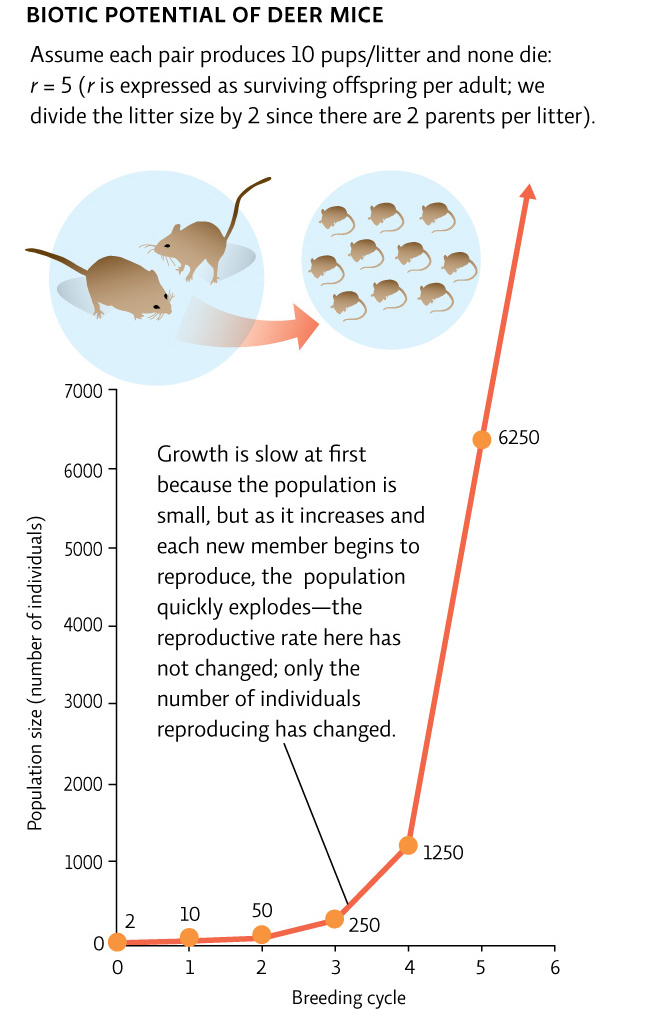
Populations that have a high biotic potential have high fecundity (females typically produce lots of offspring), and reach reproductive maturity quickly. The higher the biotic potential, the faster the population of a given species will grow under ideal conditions. North American species such as deer mice and the invasive spotted knapweed have higher biotic potential than species such as grizzly bears and spruce trees.
Exponential growth is typically seen when a species first enters a new environment, or if there is an influx of new resources. The population must have a high birth rate—most individuals must have access to enough food, water, and habitat in which to reproduce—and a low death rate. The loss of predators can also lead to exponential growth among their prey species.
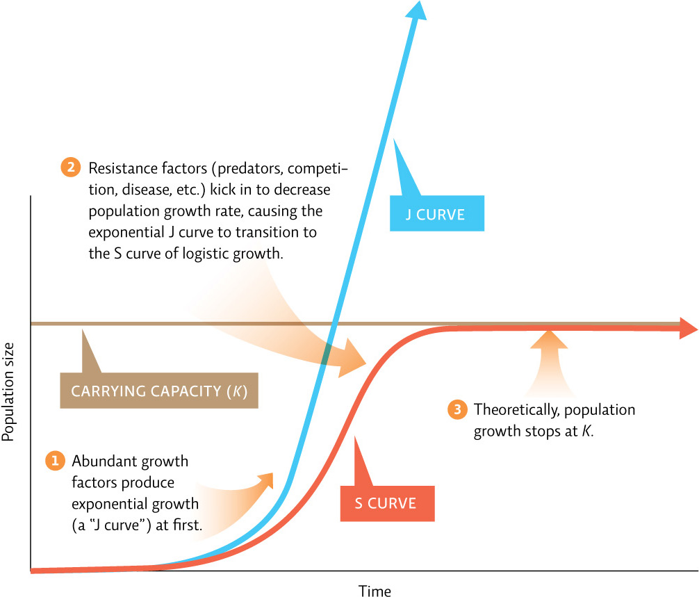
A population that is growing exponentially will have a J-shaped curve if plotted on a graph with time on the x-axis and population size on the y-axis. The J curve shows a slight lag at first and then a rapid increase. This is due to the fact that the larger the population, the faster it grows, even at the same growth rate. Think of it this way: doubling a small number yields a number that is still small. Doubling a large number, on the other hand, produces a very large number.
As an example of how profound exponential growth can be, imagine someone gave you a dollar one day and then, each subsequent day for a month, doubled the amount given to you the previous day. On day 1 you would have 1 dollar; on day 2 you would be given 2 dollars; on day 3 you’d be given 4 dollars, and on day 4, you would be given 8 dollars. By day 31, you would have over $2.1 billion. Exponential growth can create large populations quickly. [infographic 7.2]
Exponential growth can’t last forever, however. As a population begins to fill its environment, its growth rate decreases, because as more individuals use the available resources, the resources become scarce. Some individuals starve or are unable to find habitat in which to reproduce, and crowding may also bring about an increase in disease and aggression. Predation pressure may increase as the more numerous prey are easier to track and capture or simply because the predator population itself has increased. This kind of growth—in which as population size increases, growth rate decreases—is called logistic growth. A population that grows logistically will produce an S-shaped curve if plotted on a graph with time on the x-axis and population size on the y-axis. The S is created by the initial exponential growth (just like the first part of the J-shaped curve), followed by decelerating growth as the species approaches its maximum sustainable population size, where it levels off.
119
The population size that a particular environment can support indefinitely—without long-term damage to the environment—is called its carrying capacity, signified as K in population models. Carrying capacity depends on the presence of growth factors (resources needed for species to survive or reproduce) and it varies among species; the same environment can support many more mice than wolves, for example. Over time, a population’s carrying capacity can change. If resources are diminished at a faster rate than they are replenished, the carrying capacity will drop. If, on the other hand, new resources are added or become available, perhaps due to the loss of a competitor, the carrying capacity for a species may rise. [infographic 7.3]