Regression equations
When a plot shows a straight-line relationship as strong as that in Figure 15.1, it is easy to draw a line close to the points by eye. In Figure 15.2, however, different people might draw quite different lines by eye. Because we want to predict y from x, we want a line that is close to the points in the vertical (y) direction. It is hard to concentrate on just the vertical distances when drawing a line by eye. What is more, drawing by eye gives us a line on the graph but not an equation for the line. We need a way to find from the data the equation of the line that comes closest to the points in the vertical direction. There are many ways to make the collection of vertical distances “as small as possible.” The most common is the least-squares method.
Least-squares regression line
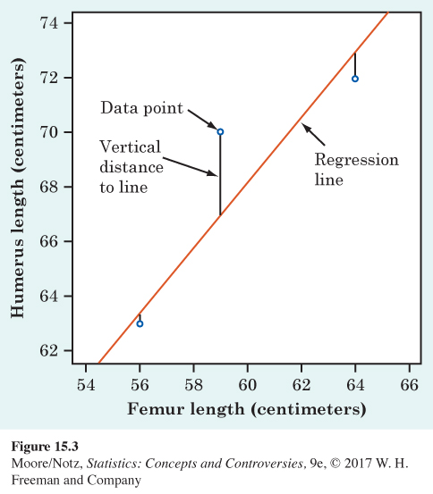
The least-squares regression line of y on x is the line that makes the sum of the squares of the vertical distances of the data points from the line as small as possible.
Figure 15.3 illustrates the least-squares idea. This figure magnifies the center part of Figure 15.1 to focus on three of the points. We see the vertical distances of these three points from the regression line. To find the least-squares line, look at these vertical distances (all five for the fossil data), square them, and move the line until the sum of the squares is the smallest it can be for any line. The lines drawn on the scatterplots in Figures 15.1 and 15.2 are the least-squares regression lines. We won’t give the formula for finding the least-squares line from data—that’s a job for a calculator or computer. You should, however, be able to use the equation that the machine produces.
343
In writing the equation of a line, x stands as usual for the explanatory variable and y for the response variable. The equation of a line has the form
y = a + bx
The number b is the slope of the line, the amount by which y changes when x increases by one unit. The number a is the intercept, the value of y when x = 0. To use the equation for prediction, just substitute your x-value into the equation and calculate the resulting y-value.
EXAMPLE 3 Using a regression equation
In Example 1, we used the “up-and-over” method in Figure 15.1 to predict the humerus length for a fossil whose femur length is 50 cm. The equation of the least-squares line is
humerus length = −3.66 + (1.197 × femur length)
The slope of this line is b = 1.197. This means that for these fossils, humerus length goes up by 1.197 cm when femur length goes up 1 cm. The slope of a regression line is usually important for understanding the data. The slope is the rate of change, the amount of change in the predicted y when x increases by 1.
344
The intercept of the least-squares line is a = −3.66. This is the value of the predicted y when x = 0. Although we need the intercept to draw the line, it is statistically meaningful only when x can actually take values close to zero. Here, femur length 0 is impossible (recall that the femur is a bone in the leg), so the intercept has no statistical meaning.
To use the equation for prediction, substitute the value of x and calculate y. The predicted humerus length for a fossil with a femur 50 cm long is
humerus length = −3.66 + (1.197)(50)
= 56.2 cm
To draw the line on the scatterplot, predict y for two different values of x. This gives two points. Plot them and draw the line through them.
![]() Regression toward the mean To “regress” means to go backward. Why are statistical methods for predicting a response from an explanatory variable called “regression”? Sir Francis Galton (1822–1911), who was the first to apply regression to biological and psychological data, looked at examples such as the heights of children versus the heights of their parents. He found that the taller-than-average parents tended to have children who were also taller than average, but not as tall as their parents. Galton called this fact “regression toward the mean,” and the name came to be applied to the statistical method.
Regression toward the mean To “regress” means to go backward. Why are statistical methods for predicting a response from an explanatory variable called “regression”? Sir Francis Galton (1822–1911), who was the first to apply regression to biological and psychological data, looked at examples such as the heights of children versus the heights of their parents. He found that the taller-than-average parents tended to have children who were also taller than average, but not as tall as their parents. Galton called this fact “regression toward the mean,” and the name came to be applied to the statistical method.
NOW IT’S YOUR TURN
Question 15.1
15.1 Fossil bones. Use the equation of the least-squares line
humerus length = −3.66 + (1.197 × femur length)
to predict the humerus length for a fossil with a femur 70 cm long.