Correlation and regression
Correlation measures the direction and strength of a straight-line relationship. Regression draws a line to describe the relationship. Correlation and regression are closely connected, even though regression requires choosing an explanatory variable and correlation does not.
346
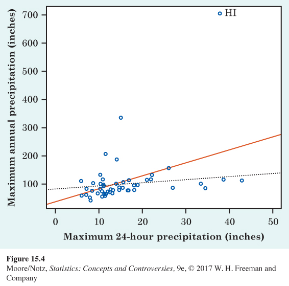
Both correlation and regression are strongly affected by outliers. Be wary if your scatterplot shows strong outliers. Figure 15.4 plots the record-high yearly precipitation in each state against that state’s record-high 24-hour precipitation. Hawaii is a high outlier, with a yearly record of 704.83 inches of rain recorded at Kukui in 1982. The correlation for all 50 states in Figure 15.4 is 0.510. If we leave out Hawaii, the correlation drops to r = 0.248. The solid line in the figure is the least-squares line for predicting the annual record from the 24-hour record. If we leave out Hawaii, the least-squares line drops down to the dotted line. This line is nearly flat—there is little relation between yearly and 24-hour record precipitation once we decide to ignore Hawaii.
The usefulness of the regression line for prediction depends on the strength of the association. That is, the usefulness of a regression line depends on the correlation between the variables. It turns out that the square of the correlation is the right measure.
r2 in regression
The square of the correlation, r2, is the proportion of the variation in the values of y that is explained by the least-squares regression of y on x.
347
The idea is that when there is a straight-line relationship, some of the variation in y is accounted for by the fact that as x changes, it pulls y along with it.
EXAMPLE 5 Using r2
Look again at Figure 15.1. There is a lot of variation in the humerus lengths of these five fossils, from a low of 41 cm to a high of 84 cm. The scatterplot shows that we can explain almost all of this variation by looking at femur length and at the regression line. As femur length increases, it pulls humerus length up with it along the line. There is very little leftover variation in humerus length, which appears in the scatter of points about the line. Because r = 0.994 for these data, r2 = (0.994)2 = 0.988. So, the variation “along the line” as femur length pulls humerus length with it accounts for 98.8% of all the variation in humerus length. The scatter of the points about the line accounts for only the remaining 1.2%. Little leftover scatter says that prediction will be accurate.
![]() Did the vote counters cheat? Republican Bruce Marks was ahead of Democrat William Stinson when the voting-machines results were tallied in their 1993 Pennsylvania election. But Stinson was ahead after absentee ballots were counted by the Democrats, who controlled the election board. A court fight followed. The court called in a statistician, who used regression with data from past elections to predict the counts of absentee ballots from the voting-machines results. Marks’s lead of 564 votes from the machines predicted that he would get 133 more absentee votes than Stinson. In fact, Stinson got 1025 more absentee votes than Marks. Did the vote counters cheat?
Did the vote counters cheat? Republican Bruce Marks was ahead of Democrat William Stinson when the voting-machines results were tallied in their 1993 Pennsylvania election. But Stinson was ahead after absentee ballots were counted by the Democrats, who controlled the election board. A court fight followed. The court called in a statistician, who used regression with data from past elections to predict the counts of absentee ballots from the voting-machines results. Marks’s lead of 564 votes from the machines predicted that he would get 133 more absentee votes than Stinson. In fact, Stinson got 1025 more absentee votes than Marks. Did the vote counters cheat?
Contrast the voting data in Figure 15.2. There is still a straight-line relationship between the 1980 and 1984 Democratic votes, but there is also much more scatter of points about the regression line. Here, r = 0.704 and so r2 = 0.496. Only about half the observed variation in the 1984 Democratic vote is explained by the straight-line pattern. You would still guess a higher 1984 Democratic vote for a state that was 45% Democratic in 1980 than for a state that was only 30% Democratic in 1980. But lots of variation remains in the 1984 votes of states with the same 1980 vote. That is the other half of the total variation among the states in 1984. It is due to other factors, such as differences in the main issues in the two elections and the fact that President Reagan’s two Democratic opponents came from different parts of the country.
In reporting a regression, it is usual to give r2 as a measure of how successful the regression was in explaining the response. When you see a correlation, square it to get a better feel for the strength of the association. Perfect correlation (r = −1 or r = 1) means the points lie exactly on a line. Then, r2 = 1 and all of the variation in one variable is accounted for by the straight-line relationship with the other variable. If r = −0.7 or r = 0.7, r2 = 0.49 and about half the variation is accounted for by the straight-line relationship. In the r2 scale, correlation ±0.7 is about halfway between 0 and ±1.
348
NOW IT’S YOUR TURN
ex15-02
Question 15.2
15.2 At the ballpark. Table 14.2 (page 336) gives data on the prices charged for for beer (per ounce) and for a hot dog at Major League Baseball stadiums. The correlation between the prices is r = 0.36. What proportion of the variation in hot dog prices is explained by the least-squares regression of hot dog prices on beer prices (per ounce)?