The question of causation

There is a strong relationship between cigarette smoking and death rate from lung cancer. Does smoking cigarettes cause lung cancer? There is a strong association between the availability of handguns in a nation and that nation’s homicide rate from guns. Does easy access to handguns cause more murders? It says right on the pack that cigarettes cause cancer. Whether more guns cause more murders is hotly debated. Why is the evidence for cigarettes and cancer better than the evidence for guns and homicide?
We already know three big facts about statistical evidence for cause and effect.
Statistics and causation
1. A strong relationship between two variables does not always mean that changes in one variable cause changes in the other.
2. The relationship between two variables is often influenced by other variables lurking in the background.
3. The best evidence for causation comes from randomized comparative experiments.

EXAMPLE 6 Does television extend life?
Measure the number of television sets per person x and the life expectancy y for the world’s nations. There is a high positive correlation: nations with many TV sets have higher life expectancies.
349
The basic meaning of causation is that by changing x we can bring about a change in y. Could we lengthen the lives of people in Botswana by shipping them TV sets? No. Rich nations have more TV sets than poor nations. Rich nations also have longer life expectancies because they offer better nutrition, clean water, and better health care. There is no cause-and-effect tie between TV sets and length of life.
Example 6 illustrates our first two big facts. Correlations such as this are sometimes called “nonsense correlations.” The correlation is real. What is nonsense is the conclusion that changing one of the variables causes changes in the other. A lurking variable—such as national wealth in Example 6—that influences both x and y can create a high correlation even though there is no direct connection between x and y. We might call this common response: both the explanatory and the response variable are responding to some lurking variable.
EXAMPLE 7 Obesity in mothers and daughters
What causes obesity in children? Inheritance from parents, overeating, lack of physical activity, and too much television have all been named as explanatory variables.
The results of a study of Mexican American girls aged 9 to 12 years are typical. Researchers measured body mass index (BMI), a measure of weight relative to height, for both the girls and their mothers. People with high BMI are overweight or obese. They also measured hours of television watched, minutes of physical activity, and intake of several kinds of food. The result: the girls’ BMIs were weakly correlated with physical activity (r = −0.18), diet, and television. The strongest correlation (r = 0.506) was between the BMI of daughters and the BMI of their mothers.
Body type is in part determined by heredity. Daughters inherit half their genes from their mothers. There is, therefore, a direct causal link between the BMI of mothers and daughters. Of course, the causal link is far from perfect. The mothers’ BMIs explain only 25.6% (that’s again) of the variation among the daughters’ BMIs. Other factors, some measured in the study and others not measured, also influence BMI. Even when direct causation is present, it is rarely a complete explanation of an association between two variables.
350
Can we use or from Example 7 to say how much inheritance contributes to the daughters’ BMIs? No. Remember confounding. It may well be that mothers who are overweight also set an example of little exercise, poor eating habits, and lots of television. Their daughters pick up these habits to some extent, so the influence of heredity is mixed up with influences from the girls’ environment. We can’t say how much of the correlation between mother and daughter BMIs is due to inheritance.
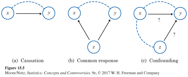
Figure 15.5 shows in outline form how a variety of underlying links between variables can explain association. The dashed line represents an observed association between the variables and . Some associations are explained by a direct cause-and-effect link between the variables. The first diagram in Figure 15.5 shows “ causes ” by an arrow running from to . The second diagram illustrates common response. The observed association between the variables and is explained by a lurking variable . Both and change in response to changes in . This common response creates an association even though there may be no direct causal link between and . The third diagram in Figure 15.5 illustrates confounding. Both the explanatory variable and the lurking variable may influence the response variable . Variables and are themselves associated, so we cannot distinguish the influence of from the influence of . We cannot say how strong the direct effect of on is. In fact, it can be hard to say if influences at all.
In Example 7, there is a causal link between the BMI of mothers and daughters. However, other factors, some measured in the study and some not measured, also influence the BMI of daughters. This is an example of confounding, illustrated in Figure 15.5(c). The in the figure corresponds to the BMI of the mother, the to one of the other factors, and the to the BMI of the daughter.
351
Both common response and confounding involve the influence of a lurking variable or variables on the response variable . We won’t belabor the distinction between the two kinds of relationships. Just remember that “beware the lurking variable” is good advice in thinking about relationships between variables. Here is another example of common response, in a setting where we want to do prediction.
EXAMPLE 8 SAT scores and college grades
High scores on the SAT examinations in high school certainly do not cause high grades in college. The moderate association ( is about 27%) is no doubt explained by common response variables such as academic ability, study habits, and staying sober. Figure 15.5(b) illustrates this. In the figure, might correspond to academic ability, to SAT scores, and to grades in college.
The ability of SAT scores to partly predict college performance doesn’t depend on causation. We need only believe that the relationship between SAT scores and college grades that we see in past years will continue to hold for this year’s high school graduates. Think once more of our fossils, where femur length predicts humerus length very well. The strong relationship is explained by common response to the overall age and size of the beasts whose fossils we now examine. Prediction doesn’t require causation.
352
Discussion of these examples has brought to light two more big facts about causation:
STATISTICAL CONTROVERSIES
Gun Control and Crime
Do strict controls on guns, especially handguns, reduce crime? To many people, the answer must be “Yes.” More than half of all murders in the United States are committed with handguns. The U.S. murder rate (per 100,000 population) is 1.7 times that of Canada, and the rate of murders with handguns is 15 times higher. Surely guns help bad things happen. Then John Lott, a University of Chicago economist, did an elaborate statistical study using data from all 3054 counties in the United States over the 18-year period from 1977 to 1994. Lott found that as states relaxed gun laws to allow adults to carry guns, the crime rate dropped. He argued that guns reduce crime by allowing citizens to defend themselves and by making criminals hesitate.
Lott used regression methods to determine the relationship between crime and many explanatory variables and to isolate the effect of permits to carry concealed guns after adjusting for other explanatory variables. You can find a link to a copy of Lott’s study at www2.lib.uchicago.edu/~llou/guns.html.
The resulting debate, still going on, has been loud. People feel strongly about gun control. Most reacted to Lott’s work based on whether or not they liked his conclusion. Gun supporters painted Lott as Moses revealing truth at last; opponents knew he must be both wrong and evil.
Is Lott right? What do you see as the weaknesses of his study based on what you have learned about statistics?
More about statistics and causation
4. The observed relationship between two variables may be due to direct causation, common response, or confounding. Two or more of these factors may be present together.
5. An observed relationship can, however, be used for prediction without worrying about causation as long as the patterns found in past data continue to hold true.
NOW IT’S YOUR TURN
Question 15.3
15.3 At the ballpark. Table 14.2 (page 336) gives data on the prices charged for beer (per ounce) and for a hot dog at Major League Baseball stadiums. The correlation between the prices is . Do you think the observed relationship is due to direct causation, common response, confounding, or some combination of these? Explain your answer.