Estimating with confidence
We want to estimate the proportion p of the individuals in a population who have some characteristic—they are employed, or they approve the president’s performance, for example. Let’s call the characteristic we are looking for a “success.’’ We use the proportion of successes in a simple random sample (SRS) to estimate the proportion p of successes in the population. How good is the statistic as an estimate of the parameter p? To find out, we ask, “What would happen if we took many samples?’’ Well, we know that would vary from sample to sample. We also know that this sampling variability isn’t haphazard. It has a clear pattern in the long run, a pattern that is pretty well described by a Normal curve. Here are the facts.
Sampling distribution of a sample proportion
The sampling distribution of a statistic is the distribution of values taken by the statistic in all possible samples of the same size from the same population.
Take an SRS of size n from a large population that contains proportion p of successes. Let be the sample proportion of successes,
496
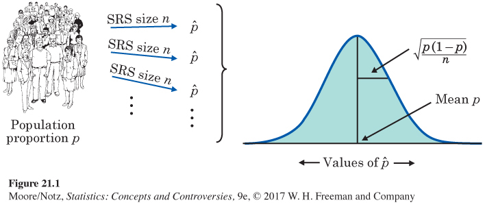
Then, if the sample size is large enough:
• The sampling distribution of is approximately Normal.
• The mean of the sampling distribution is p.
• The standard deviation of the sampling distribution is
These facts can be proved by mathematics, so they are a solid starting point. Figure 21.1 summarizes them in a form that also reminds us that a sampling distribution describes the results of lots of samples from the same population.
Standard error
The standard deviation of the sampling distribution of a sample statistic is commonly referred to as the standard error.
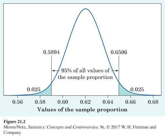
EXAMPLE 2 More on soda consumption
Suppose, for example, that the truth is that 62% of Americans actively tried to avoid drinking regular soda or pop in 2015. Then, in the setting of Example 1, p = 0.62. The Gallup sample of size n = 1009 would, if repeated many times, produce sample proportions that closely follow the Normal distribution with
mean = p = 0.62
497
and

The center of this Normal distribution is at the truth about the population. That’s the absence of bias in random sampling once again. The standard error is small because the sample is quite large. So, almost all samples will produce a statistic that is close to the true p. In fact, the 95 part of the 68–95–99.7 rule says that 95% of all sample outcomes will fall between
mean − 2 standard errors = 0.62 − 0.0306 = 0.5894
and
mean + 2 standard errors = 0.62 + 0.0306 = 0.6506
Figure 21.2 displays these facts.
498
So far, we have just put numbers on what we already knew: we can trust the results of large random samples because almost all such samples give results that are close to the truth about the population. The numbers say that in 95% of all samples of size 1009, the statistic and the parameter p are within 0.0306 of each other. We can put this another way: 95% of all samples give an outcome such that the population truth p is captured by the interval from to .
The 0.03 came from substituting p = 0.62 into the formula for the standard error of . For any value of p, the general fact is:
When the population proportion has the value p, 95% of all samples catch p in the interval extending 2 standard errors on either side of .
That’s the interval
Is this the 95% confidence interval we want? Not quite. The interval can’t be found just from the data because the standard deviation involves the population proportion p, and in practice, we don’t know p. In Example 2, we used p = 0.62 in the formula, but this may not be the true p.
What can we do? Well, the standard deviation of the statistic , or the standard error, does depend on the parameter p, but it doesn’t change a lot when p changes. Go back to Example 2 and redo the calculation for other values of p. Here’s the result:
| Value of p: | 0.60 | 0.61 | 0.62 | 0.63 | 0.64 |
| Standard error: | 0.01542 | 0.01535 | 0.01528 | 0.01520 | 0.01511 |
We see that, if we guess a value of p reasonably close to the true value, the standard error found from the guessed value will be about right. We know that, when we take a large random sample, the statistic is almost always close to the parameter p. So, we will use as the guessed value of the unknown p. Now we have an interval that we can calculate from the sample data.
95% confidence interval for a proportion
Choose an SRS of size n from a large population that contains an unknown proportion p of successes. Call the proportion of successes in this sample . An approximate 95% confidence interval for the parameter p is
499
![]() Who is a smoker? When estimating a proportion p, be sure you know what counts as a “success.’’ The news says that 20% of adolescents smoke. Shocking. It turns out that this is the percentage who smoked at least once in the past month. If we say that a smoker is someone who smoked in at least 20 of the past 30 days and smoked at least half a pack on those days, fewer than 4% of adolescents qualify.
Who is a smoker? When estimating a proportion p, be sure you know what counts as a “success.’’ The news says that 20% of adolescents smoke. Shocking. It turns out that this is the percentage who smoked at least once in the past month. If we say that a smoker is someone who smoked in at least 20 of the past 30 days and smoked at least half a pack on those days, fewer than 4% of adolescents qualify.
EXAMPLE 3 A confidence interval for soda consumption
The Gallup random sample of 1009 adult Americans found that 616 reported actively trying to avoid drinking regular soda or pop in 2015, a sample proportion . The 95% confidence interval for the proportion of all Americans who actively tried to avoid drinking regular soda or pop in 2015 is
= 0.611 ± (2)(0.01535)
= 0.611 ± 0.0307
= 0.5803 to 0.6417
Interpret this result as follows: we got this interval by using a recipe that catches the true unknown population proportion in 95% of all samples. The shorthand is: we are 95% confident that the true proportion of all Americans who actively tried to avoid drinking regular soda or pop in 2015 lies between 58.03% and 64.17%.
NOW IT’S YOUR TURN
Question 21.1
21.1 Gambling. A May 2011 Gallup Poll consisting of a random sample of 1018 adult Americans found that 31% believe gambling is morally wrong. Find a 95% confidence interval for the proportion of all adult Americans who believe gambling is morally wrong. How would you interpret this interval?