Understanding confidence intervals
Our 95% confidence interval for a population proportion has the familiar form
estimate ± margin of error
News reports of sample surveys, for example, usually give the estimate and the margin of error separately: “A new Gallup Poll shows that 65% of women favor new laws restricting guns. The margin of error is plus or minus four percentage points.’’ News reports usually leave out the level of confidence, although it is almost always 95%.
The next time you hear a report about the result of a sample survey, consider the following. If most confidence intervals reported in the media have a 95% level of confidence, then in about 1 in 20 poll results that you hear about, the confidence interval does not contain the true proportion.
500
Here’s a complete description of a confidence interval.
Confidence interval
A level C confidence interval for a parameter has two parts:
• An interval calculated from the data.
• A confidence level C, which gives the probability that the interval will capture the true parameter value in repeated samples.
There are many recipes for statistical confidence intervals for use in many situations. Not all confidence intervals are expressed in the form “estimate ± margin of error.’’ Be sure you understand how to interpret a confidence interval. The interpretation is the same for any recipe, and you can’t use a calculator or a computer to do the interpretation for you.
Confidence intervals use the central idea of probability: ask what would happen if we were to repeat the sampling many times. The 95% in a 95% confidence interval is a probability, the probability that the method produces an interval that does capture the true parameter.
EXAMPLE 4 How confidence intervals behave
The Gallup sample of 1009 adult Americans in 2015 found that 616 reported actively trying to avoid drinking regular soda or pop, so the sample proportion was
and the 95% confidence interval was
Draw a second sample from the same population. It finds that 700 of its 1009 respondents reported actively trying to avoid drinking regular soda or pop. For this sample,
501
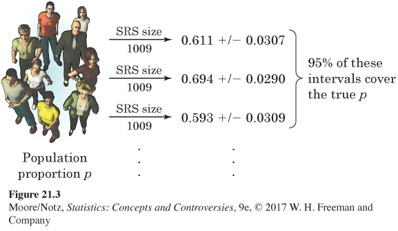
Draw another sample. Now the count is 598 and the sample proportion and confidence interval are
Keep sampling. Each sample yields a new estimate and a new confidence interval. If we sample forever, 95% of these intervals capture the true parameter. This is true no matter what the true value is. Figure 21.3 summarizes the behavior of the confidence interval in graphical form.
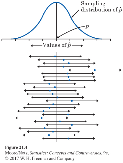
Example 4 and Figure 21.3 remind us that repeated samples give different results and that we are guaranteed only that 95% of the samples give a correct result. On the assumption that two pictures are better than one, Figure 21.4 gives a different view of how confidence intervals behave. Figure 21.4 goes behind the scenes. The vertical line is the true value of the population proportion p. The Normal curve at the top of the figure is the sampling distribution of the sample statistic , which is centered at the true p. We are behind the scenes because, in real-world statistics, we usually don’t know p.
The 95% confidence intervals from 25 SRSs appear below the graph in Figure 21.4, one after the other. The central dots are the values of , the centers of the intervals. The arrows on either side span the confidence interval. In the long run, 95% of the intervals will cover the true p and 5% will miss. Of the 25 intervals in Figure 21.4, there are 24 hits and 1 miss. (Remember that probability describes only what happens in the long run—we don’t expect exactly 95% of 25 intervals to capture the true parameter.)
502
Don’t forget that our interval is only approximately a 95% confidence interval. It isn’t exact for two reasons. The sampling distribution of the sample proportion isn’t exactly Normal. And we don’t get the standard deviation, or the standard error, of exactly right because we used in place of the unknown p. We use a new estimate of the standard deviation of the sampling distribution every time, even though the true standard deviation never changes. Both of these difficulties go away as the sample size n gets larger. So, our recipe is good only for large samples. What is more, the recipe assumes that the population is really big—at least 10 times the size of the sample. Professional statisticians use more elaborate methods that take the size of the population into account and work even for small samples. But our method works well enough for many practical uses. More important, it shows how we get a confidence interval from the sampling distribution of a statistic. That’s the reasoning behind any confidence interval.