Tests for a population mean*
The reasoning that leads to significance tests for hypotheses about a population mean μ follows the reasoning that leads to tests about a population proportion p. The big idea is to use the sampling distribution that the sample mean would have if the null hypothesis were true. Locate the value of from your data on this distribution, and see if it is unlikely. A value of that would rarely appear if H0 were true is evidence that H0 is not true. The four steps are also similar to those in tests for a proportion. Here are two examples, the first one-
EXAMPLE 4 Length of human pregnancies
Researchers have recently begun to question the actual length of a human pregnancy. According to a report published on August 6, 2013, although women are typically given a delivery date that is calculated as 280 days after the onset of their last menstrual period, only 4% of women deliver babies at 280 days. A more likely average time from ovulation to birth may be much less than 280 days. To test this theory, a random sample of 95 women with healthy pregnancies is monitored from ovulation to birth. The mean length of pregnancy is found to be days, with a standard deviation of s = 10 days. Is this sample result good evidence that the mean length of a healthy pregnancy for all women is less than 280 days?
The hypotheses. The researcher’s claim is that the mean length of pregnancy is less than 280 days. That’s our alternative hypothesis, the statement we seek evidence for. The hypotheses are
H0: μ = 280
Ha: μ < 280

532
The sampling distribution. If the null hypothesis is true, the sample mean has approximately the Normal distribution with mean μ = 280 and standard error
We once again use the sample standard deviation s in place of the unknown population standard deviation σ.
The data. The researcher’s sample gave . The standard score, or test statistic, for this outcome is
That is, the sample result is about 4.85 standard errors below the mean we would expect if, on the average, healthy pregnancies lasted for 280 days.
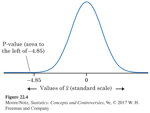
The P-value. Figure 22.4 locates the sample outcome −4.85 (in the standard scale) on the Normal curve that represents the sampling distribution if H0 is true. This curve has mean 0 and standard deviation 1 because we are using the standard scale. The P-value for our one-
533
The conclusion. A P-value of less than 0.0003 is strong evidence that the mean length of a healthy human pregnancy is below the commonly reported length of 280 days.
![]() Catching cheaters Lots of students take a long multiple-
Catching cheaters Lots of students take a long multiple-
EXAMPLE 5 Time spent eating
The Bureau of Labor Statistics conducts the American Time Use Survey (ATUS). This survey is intended to provide nationally representative estimates of how, where, and with whom Americans spend their time, and more than 159,000 individuals have been surveyed between 2003 and 2014. In 2014, it was reported that Americans spend an average of 1.23 hours per day eating and drinking. An administrator at a college campus in Ohio conducts a survey of a random sample of 150 college students and finds that the average amount of time these students report eating and drinking per day is hours, with a standard deviation of s = 0.25 hour. Is this evidence that the college students eat and drink, on average, a different amount of time each day when compared to the general population?

The hypotheses. The null hypothesis is “no difference’’ from the national mean. The alternative is two-
H0: μ = 1.23
Ha: μ ≠ 1.23
The sampling distribution. If the null hypothesis is true, the sample mean has approximately the Normal distribution with mean μ = 1.23 and standard error
The data. The sample mean is . The standard score, or test statistic, for this outcome is
534
We know that an outcome 1 standard error away from the mean of a Normal distribution is not very surprising. The last step is to make this formal.
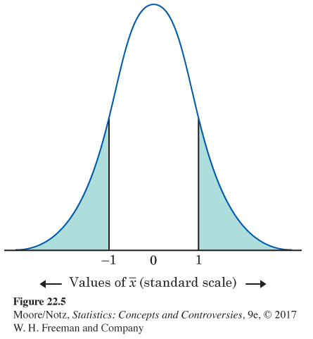
The P-value. Figure 22.5 locates the sample outcome 1 (in the standard scale) on the Normal curve that represents the sampling distribution if H0 is true. The two-
The conclusion. The large P-value gives us no reason to think that the mean time spent eating and drinking per day among the Ohio college students differs from the national average.
The test assumes that the 150 students in the sample are an SRS from the population of all college students. We should check this assumption by asking how the data were produced. If the data come from a survey conducted on one particular day, in one dining hall on campus, for example, the data are of little value for our purpose. It turns out that the college administrator attempted to gather a random sample by using a computer program to randomly select names from a college directory. He then sent surveys out to those students who had been chosen to participate in this study of eating habits.
535
What if the college administrator did not draw a random sample? You should be very cautious about inference based on nonrandom samples, such as convenience samples or random samples with large nonresponse. Although it is possible for a convenience sample to be representative of the population and, hence, yield reliable inference, establishing this is not easy. You must be certain that the method for selecting the sample is unrelated to the quantity being measured. You must make a case that individuals are independent. You must use additional information to argue that the sample is representative. This can involve comparing other characteristics of the sample to known characteristics of the population. Is the proportion of men and women in the sample about the same as in the population? Is the racial composition of the sample about the same as in the population? What about the distribution of ages or other demographic characteristics? Even after arguing that your sample appears to be representative, the case is not as compelling as that for a truly random sample. You should proceed with caution.
The data in Example 5 do not establish that the mean time spent eating and drinking μ for this sample of college students is 1.23 hours. We sought evidence that μ differed from 1.23 hours and failed to find convincing evidence. That is all we can say. No doubt the mean time spent eating and drinking among the entire college population is not exactly equal to 1.23 hours. A large enough sample would give evidence of the difference, even if it is very small.
NOW IT’S YOUR TURN
Question 22.3
22.3 IQ scores. The mean IQ for the entire population in any age group is supposed to be 100. Suppose that we measure the IQ of 31 seventh-
*This section is optional.