Chapter 24: Two-Way Tables and the Chi-Square Test*

Inference for a two-way table

We often gather data and arrange them in a two-way table to see if two categorical variables are related to each other. The sample data are easy to investigate: turn them into percentages and look for an association between the row and column variables. Is the association in the sample evidence of an association between these variables in the entire population? Or could the sample association easily arise just from the luck of random sampling? This is a question for a significance test.

EXAMPLE 3 Treating cocaine addiction

Cocaine addicts need the drug to feel pleasure. Perhaps giving them a medication that fights depression will help them resist cocaine. A three-year study compared an antidepressant called desipramine, lithium (a standard treatment for cocaine addiction), and a placebo. The subjects were 72 chronic users of cocaine who wanted to break their drug habit. An equal number of the subjects were randomly assigned to each treatment. Here are the counts and percentages of the subjects who succeeded in not using cocaine during the study:

Group	Treatment	Subjects	Successes	Percent
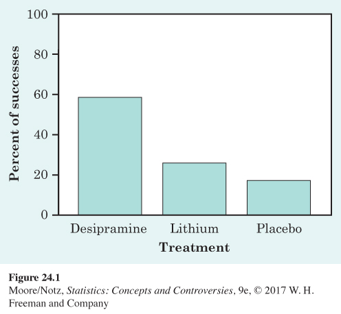
1	Desipramine	24	14	58.3
2	Lithium	24	6	25.0
3	Placebo	24	4	16.7

Lawrence Manning/CORBIS

The sample proportions of subjects who did not use cocaine are quite different. In particular, the percentage of subjects in the desipramine group who did not use cocaine was much higher than for the lithium or placebo group. The bar graph in Figure 24.1 compares the results visually. Are these data good evidence that there is a relationship between treatment and outcome in the population of all cocaine addicts?

The test that answers this question starts with a two-way table. Here’s the table for the data of Example 3:

	Success	Failure	Total
Desipramine	14	10	24
Lithium	6	18	24
Placebo	4	20	24
Total	24	48	72

Page 575

Figure 24.1: Figure 24.1 Bar graph comparing the success rates of three treatments for cocaine addiction, Example 3.

Our null hypothesis, as usual, says that the treatments have no effect. That is, addicts do equally well on any of the three treatments. The differences in the sample are just the result of chance. Our null hypothesis is

H₀: There is no association between the treatment an addict receives and whether or not there is success in not using cocaine in the population of all cocaine addicts.

Expressing this hypothesis in terms of population parameters can be a bit complicated, so we will be content with the verbal statement. The alternative hypothesis just says, “Yes, there is some association between the treatment an addict receives and whether or not he succeeds in staying off cocaine.” The alternative doesn’t specify the nature of the relationship. It doesn’t say, for example, “Addicts who take desipramine are more likely to succeed than addicts given lithium or a placebo.”

To test H₀, we compare the observed counts in a two-way table with the expected counts, the counts we would expect—except for random variation—if H₀ were true. If the observed counts are far from the expected counts, that is evidence against H₀. We can guess the expected counts for the cocaine study. In all, 24 of the 72 subjects succeeded. That’s an overall success rate of one-third because 24/72 is one-third. If the null hypothesis is true, there is no difference among the treatments. So we expect one-third of the subjects in each group to succeed. There were 24 subjects in each group, so we expect eight successes and 16 failures in each group. If the treatment groups differ in size, the expected counts will differ also, even though we still expect the same proportion in each group to succeed. Fortunately, there is a rule that makes it easy to find expected counts. Here it is.

Page 576

Expected counts

The expected count in any cell of a two-way table when H₀ is true is

$expected count = \frac{row total \times column total}{table total}$

Try it. For example, the expected count of successes in the desipramine group is

$\begin{array}{l} expected count & = & \frac{row 1 total \times column 1 total}{table total} \\ = & \frac{(24) (24)}{72} = 8 \end{array}$

If the null hypothesis of no treatment differences is true, we expect eight of the 24 desipramine subjects to succeed. That’s just what we guessed.

NOW IT’S YOUR TURN

Question 24.1

24.1 Video-gaming and grades. The popularity of computer, video, online, and virtual reality games has raised concerns about their ability to negatively impact youth. Based on a recent survey, 1808 students aged 14 to 18 in Connecticut high schools were classified by their average grades and by whether they had or had not played such games. The following table summarizes the findings.

	Grade Average
	A’s and B’s	C’s	D’s and F’s
Played games	736	450	193
Never played games	205	144	80

Find the expected count of students with average grades of A’s and B’s who have played computer, video, online, or virtual reality games under the null hypothesis that there is no association between grades and game playing in the population of students. Assume that the sample was a random sample of students in Connecticut high schools.

24.1. The expected count of students with average grades of A and B who have played games is

$\begin{array}{l} expected count & = & \frac{row 1 total \times row 2 total}{table total} \\ = & \frac{(1379) (941)}{1808} = 717.7 \end{array}$

Page 577