10.1 Geospatial Lab Application: Remotely Sensed Imagery and Color Composites
This chapter’s lab will introduce you to some of the basics of working with multispectral remotely sensed imagery through the use of the MultiSpec software program.
Objectives
The goals to take away from this exercise are:
 to familiarize yourself with the basics of the MultiSpec software program.
- to load various bands into the color guns and examine the results.
- to create and examine different color composites.
- to compare the brightness values of distinct water and environmental features in a remotely sensed satellite image in order to create basic spectral profiles.
Obtaining Software
The current version of MultiSpec (3.3) is available for free download at https://engineering.purdue.edu/∼biehl/MultiSpec/.
Important note: Software and online resources sometimes change fast. This lab was designed with the most recently available version of the software at the time of writing. However, if the software or Websites have significantly changed between then and now, an updated version of this lab (using the newest versions) is available online at http://www.whfreeman.com/shellito2e.
Using Geospatial Technologies
The concepts you’ll be working with in this lab are used in a variety of real-world applications, including:
- environmental science, which uses satellite imagery to derive signatures for various classes of land cover, and to create accurate land cover maps.
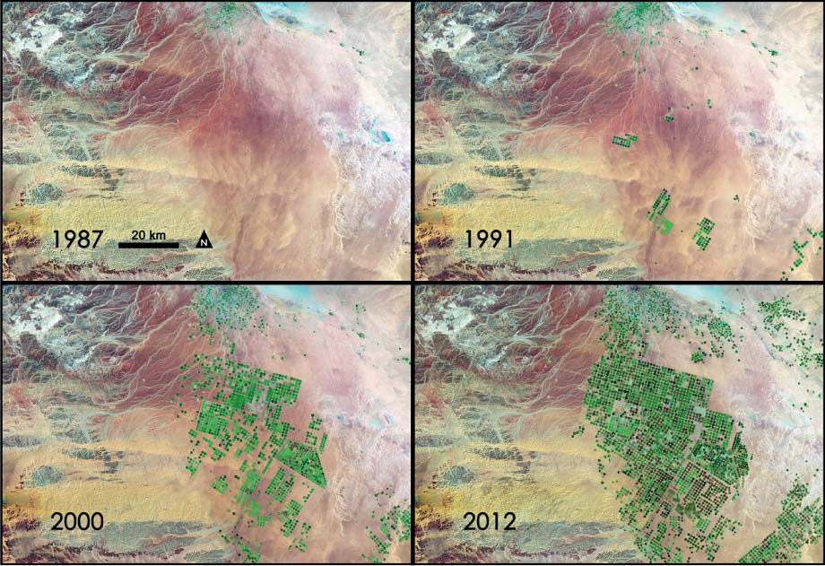
- urban planning, where satellite imagery collected over time can be used to study the expansion (and sometimes the contraction) of cities, and to evaluate proposals for commercial, industrial, and residential development.
348
Lab Data
Copy the folder Chapter10—it contains a Landsat 5 TM satellite image file Lab Datacalled ‘cle.img’ (which is a subset of a Landsat 5 TM scene from 9/11/2005 of northeast Ohio). We will discuss more about Landsat imagery in Chapter 11, but the TM imagery bands refer to the following portions of the electromagnetic (EM) spectrum in micrometers (μm):
- Band 1: Blue (0.45 to 0.52 µm)
- Band 2: Green (0.52 to 0.60 µm)
- Band 3: Red (0.63 to 0.69 µm)
- Band 4: Near infrared (0.76 to 0.90 µm)
- Band 5: Middle infrared (1.55 to 1.75 µm)
- Band 6: Thermal infrared (10.40 to 12.50 µm)
- Band 7: Middle infrared (2.08 to 2.35 µm)
Landsat TM imagery is 30-meter spatial resolution (except for the thermal-infrared band, which is 120 meters). Thus, each pixel you will be examining represents a 30 meter × 30 meter square area.
Localizing This Lab
Although this lab focuses on a section of a Landsat scene from northeast Ohio, Landsat imagery is available for download via GLOVIS at http://glovis.usgs.gov. This will provide the raw data, which will have to be imported into MultiSpec and processed to use in the program.
349
Alternatively, NASA has information for obtaining free Landsat data for use in MultiSpec online at http://change.gsfc.nasa.gov/create.html. The page provides step-by-step instructions for acquiring free data for your own area and getting it into MultiSpec format.
10.1 MultiSpec and Band Combinations
- Start MultiSpec. MultiSpec will start with an empty text box (which will give you updates and reports of processes in the program). You can minimize the text box for now.
- To get started with a remotely sensed image, select Open Image from the File pull-down menu. Alternatively, you can select the Open icon from the toolbar:
 (Source: Purdue Research Foundation)
 - Navigate to the Chapter10 folder, select cle.img as the file to open, and click Open.
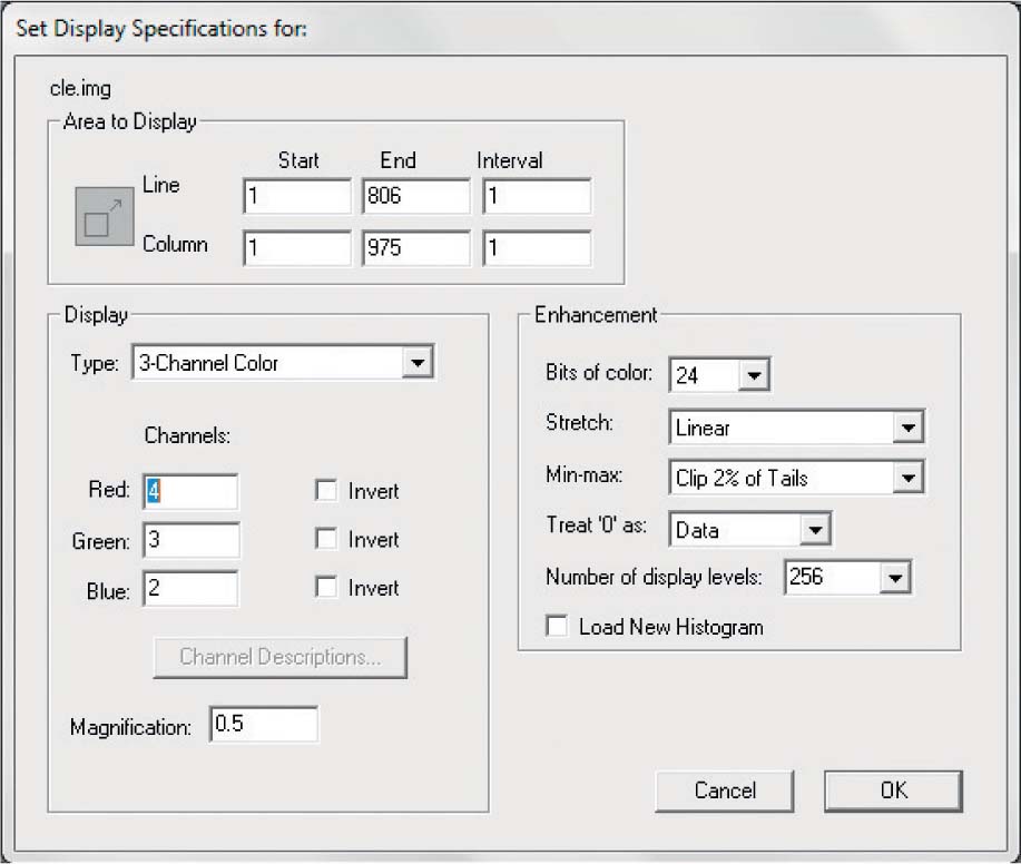
- A new dialog box will appear that allows you to set the display specification for the ‘cle’ image.
 (Source: Purdue Research Foundation)
 - Under Channels, you will see the three color guns available to you (red, green, and blue). Each color gun can hold one band (see the Lab Data section for a listing of which bands correspond to which parts of the electromagnetic spectrum). The number listed next to each color gun represents the band being displayed with that gun.
- Display band 4 in the red color gun, band 3 in the green color gun, and band 2 in the blue color gun.
- Accept the other defaults for now and click OK.
- A new window will appear and the ‘cle’ image will begin loading. This might take a minute or two to load completely.
- For the best results, maximize both MultiSpec and the window containing the ‘cle’ image. Use the bars at the edge of the window to move around the image. You can zoom in or zoom out by using the zoom tools on the toolbar:
 (Source: Purdue Research Foundation)
The large mountain icon will zoom in and the small mountain icon will zoom out. - Zoom around the image, paying attention to some of the city, landscape, and water areas.
Question 10.1
sk6ZD7sM3hjnV3q7Rug/SrWsaHF07LSGDRxBSL+jusuCERIsJMxn6UIbj3DeJxXdyCASBbnhnHiaWL2IQuestion 10.2
cwe/Ptgt1hNpROUPb8NqSfNLVdMc2Xw38EKozkQjo60s06Aw39KSKy+7OtCDS9CBHDVa9Rn4XEmT2TgLwdd4fM5+Auc1X3ZLCYJOhY3oWH2bxotQOPgyYdx5Wc4XzJjzbbJtY+5011/nxvwBKhBJ3YO5yo9B2PZEE791koPGJ5i1IFaDXvo78bQVtBcFzjwGYliNfCPTXRytrdL9jlzlqfoU3cZgSFbFd/FP2BlmYYHCGGL5/z5LtrXPp7ZsGYhryjNEzPLAqIU=Question 10.3
9ODAc+0b8oro+Ov7e3qlI3qAdoOTegw8j50npVJwA+A2uUyP4TpDF0IhWWKMwOal9Pe/o2KIRJHmCAdgQbQZ9s7QfNiZ9pppcljPtojltfkP1kjJBwAmNUK51PmN3cpO1N4bnGnTxx3wbOZn6KcqAEHDXzdgo0+J/sbAIBbJgvn36z6JrahKBhipFvHbXkOz - Reopen the image, this time using band 3 in the red gun, band 2 in the green gun, and band 1 in the blue gun (referred to as a 3-2-1 combination). Once the image reloads, pan and zoom around the image, examining the same areas you just looked at.
Question 10.4
x1AYYObgBRvRyYkgZsCEaEZuoGMGEnHoZxqM0i53u+fB/gyPSAR5A+1COFur3+T2BTqzBQr4rWdnrkCgzoSgqk+OgIuH3XfIoeWj4nmxsG+XFPbGRKhpPIYOxOW45UarvcfHv2ndiPLh/k0BOs+iUC+SYp8DidnIAJV8A/znzAfnoo7HRR8iE3Ab4Yc=Question 10.5
YK4R2hmuSHnfIpY55S2jB7E1RQmlaBRYBTziBIdHrhUOrNseGxTAkKaaFGsCb8ra1Flr3jI5ioLXTnCfUSM+keJXv1U+n95jkRN8YazMcoIuRFOnoYg/CEobPCwcpOSqMocsK6MEKlHQZnB9 - Reopen the image yet again, this time using band 2 in the red gun, band 1 in the green gun, and band 3 in the blue gun (referred to as a 2-1-3 combination). Once it reloads, pan and zoom around the image, examining the same areas you just looked at.
Question 10.6
RiglqoUU6rcsZktVZze7cU7SukohAk9Sm4+lZI2a5p6bVz0RlzKxcCO9c+vxeLAeAXbcx3Ev8QH7YqvO2/SlWQ==Question 10.7
lqQk7gsjTf8pqbwQpfRikl1rr4AKaU96zchy6uiubJ/R6C86Pc0k2zTaJKdwA5++d74qHmF8r0GAAyIN3N+feXJCVbKYwQGGTIhGINAK8eQgS3wT1qI4svkOk0rM7SETrhAO6HyGlV4aKqDE9n7pwp5/u8fc1vEx
10.2 Examining Color Composites and Color Formations
- Reopen the image one more time, returning the 4-3-2 combination (band 4 in the red gun, band 3 in the green gun, and band 2 in the blue gun). You can close the other images, as we’ll be working with this one for the rest of the lab.
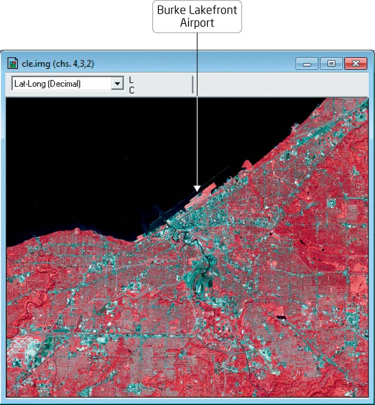
- Zoom and move around the image to find and examine Burke Lakefront Airport as follows:
 (Source: Purdue Research Foundation)
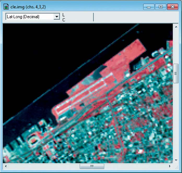
 - Zoom in to the airfield. From its shape and the pattern of the runways, you should be able to clearly identify it in the Landsat image.
 (Source: Purdue Research Foundation)
 - Examine the airfield and its surroundings.
Question 10.8
HkMuzs/GwFOJ+XvMmp3zX3WwQJVSLTahSg75Xs7tkD3zOFfYI4msUXY52Fgz5wHXocp+x6Rg3wQ= - Open a new image, this time with a 3-4-2 combination. Examine Burke Lakefront Airport in this new image and compare it to the one you’ve been working with.
Question 10.9
77QJbrfmd402FCbmqYY2laWQ6MjyxThIgR86SaLkW25n7dI1Xr4SmeWo6ohaDjvns+Thi3keVFim34TWEA79YBfdn4M= - Open another new image, this time with a 3-2-4 combination. Examine Burke Lakefront Airport in this new image and compare it with the others you’ve been working with.
Question 10.10
rj2FM7rV1HuiWn1P4XkASvlQYRkg+dVEUoT81zL5H6rOd5XtXE+VUYuKRQvNFi9Kei6oCDwamaESEPI5 - At this point, only keep the 4-3-2 image open and close the other two.
10.3 Examining Specific Brightness Values and Spectral Profiles
Regardless of how the pixels are displayed in the image, each pixel in each band of the image has a specific brightness value set in the 0–255 range. By examining those pixel values for each band, you can chart a basic ‘spectral profile’ of some features in the image.
- Zoom in to the area around Cleveland’s waterfront and identify the urban areas (in the image these will mostly be the white or cyan regions).
- From the Window pull-down menu, select New Selection Graph. Another (empty) window (called Selection Graph) will open in MultiSpec.
- In the image, locate a pixel that’s a good example of an urban or developed area. The cursor will change to a cross shape, so give the pixel one more click.
Important note: Zoom in so that you are only selecting one pixel with the cursor. - A chart will appear in the Selection Graph window that will graphically show the BVs for each band at that particular pixel (see the first page of this lab for the portions of the electromagnetic spectrum that match up with each band). The band numbers are on the x-axis and the BVs are on the y-axis. The chart can be expanded or maximized as necessary to be better able to examine the values.
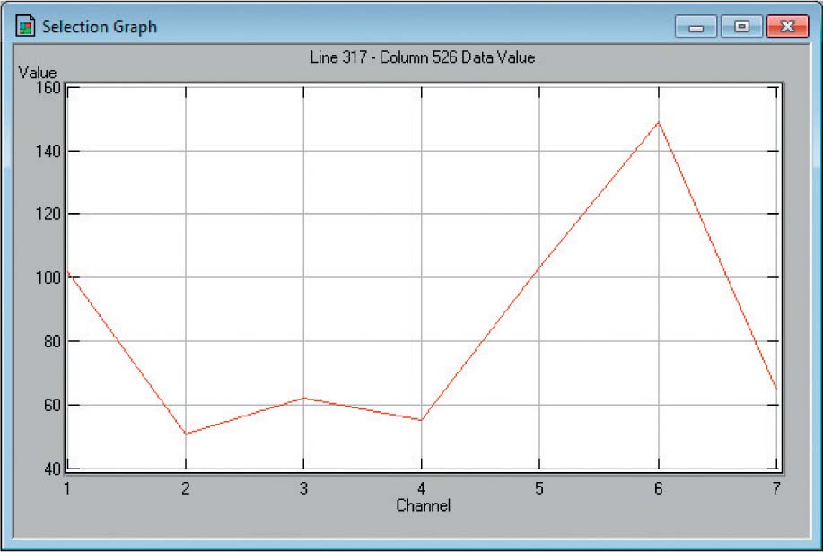 (Source: Purdue Research Foundation)
 - The Selection Graph window now shows the data that can be used to compute a simplified version of a spectral profile for an example of the particular urban land use pixel you selected from the image.
- For the next question, you’ll be required to find a pixel that’s a good example of water and another pixel that’s a good example of vegetation. You’ll also be required to translate the data from the chart to a ‘spectral profile’ for each example. In drawing the ‘profiles’ from the information on the chart, keep two things in mind:
- First, the values at the bottom of the Selection Graph window represent the numbers of the bands being examined. On the chart, the actual wavelengths of the bands are plotted out, so make sure you properly match up each band with its respective wavelength (also note that Band 6 is not being charted, since it measures emitted thermal energy rather than reflected energy like Bands 1–5 and 7).
- Second, the values on the y-axis of the Selection Graph window are BVs, not the percentage of reflection as seen in a spectral signature diagram. There are a number of factors involved with transforming BVs into the actual percent reflectance values (a BV and the percent reflectance don’t have an exact one-to-one ratio, as there are other factors that affect the measurement at the sensor, such as atmospheric effects), but in this simplified example, you’ll just chart the BV for this ‘spectral profile.’
- Examine the image for a good example of a water pixel and a vegetation pixel.
- Plot a ‘spectral profile’ diagram for the water and vegetation pixels you chose on the following diagram (remember to plot values as calculated from the BVs).
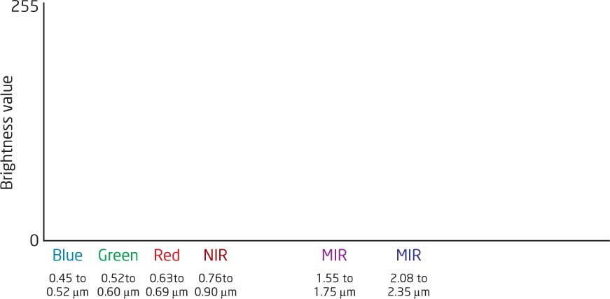
- Examine your two ‘profiles’ and answer Questions 10.11 and 10.12.
Question 10.11
JHtReW3mc8IbwnP4JiZS7kjNlN79CH+E/PbDjKSKbxkI4/EFEDGAOR3athuUtrm7Oiz3X5TKGlnGsJp+uaAhC/tCjmu5eIIVzmgLk5r1c1Bq9w4kXW8uPv+m0ml/LMpESdY9EhvF2Ay04jF5fCRiq5tZpQyyexAt4LZ6AuMNNsJQ2/mBsc1S2Kc6Cq4iGOiaAEcHYh5ATvOdr4BYNm9LGTtSiJ8syfKKHMP7XVSojBgHIptHR3k9y755CcpyLMbwvC16FvLPLRt5FiR7jsNoWgUCu04ieQppt15P5cU7BC+Rf8NgqZyMsv9dOn2cFuCzQuestion 10.12
FOLuF+MxykTO3w+p9Sb4KMK7AHwPyics39oHlKID0rtyd25Yk90Ralmf3c1dsJ8APHB+EMas3l5j8BoDKHpavAT6HrrcC0XIOB8Y2sIEvybgMmP3RVC+0YWQsEglqzUmPpjvA5zm7ufJwPoT9c1QoHg92V1Oj3sgqt+KVO4ESOCtONblCwLrILjeH/9LoaRCQga3JgXtBZ7MepT6224/yRFJldqmJ+8CNHvsQZLAipx+jsXPBTD5jSOuU+nByrFATOy3HngH+qII7VlbE920i0TZMGnKhV6iudDtYrbTmf4KBXwT93uaebTLFgJgLMUO83rSSzjClYNA4ZRJFuF/PxkEG78= - Exit MultiSpec by selecting Exit from the File pull-down menu. There’s no need to save any work in this exercise.
Closing Time
Now that you have the basics of working with remotely sensed data and examining the differences in color composites, the next two chapters will build on these skills. The Chapter 11 lab will return to using MultiSpec for more analysis of Landsat satellite imagery.