13.1 Geospatial Lab Application: Digital Terrain Analysis

This chapter’s lab will introduce you to some of the basics of digital terrain modeling—working with DEMs, contours, and imagery draped over the terrain model. You’ll be using Google Earth and the MICRODEM software program (developed by Professor Peter Guth of the Oceanography Department of the U.S. Naval Academy) for this lab.

Objectives

The goals of this lab are:

• to examine pseudo-3D terrain and to navigate across it in Google Earth.
• to create an animation that simulates flight over 3D terrain in Google Earth.
• to examine the effects of different levels of vertical exaggeration on the terrain.
• to familiarize yourself with the MICRODEM operating environment.
• to drape an image over the terrain in Google Earth.
• to derive hillshades, contours, and slope measurements from a DEM for terrain analysis.
• to examine a DEM in both 2D and perspective view.
• to use a DEM to create a flight path for a video in MICRODEM.

Using Geospatial Technologies

The concepts you’ll be working with in this lab are used in a variety of real-world applications, including:

• civil engineering, in which slope calculations from digital elevation models are utilized to aid in determining the direction of overland water flow, a process that contributes to calculating the boundaries of a watershed.
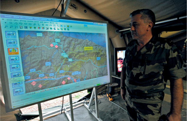
• military intelligence, which makes use of terrain maps and digital elevation models in order to have the best possible layout of real-world areas (as opposed to two-dimensional maps) when planning operations involving troop deployments, artillery placements, or drone strikes.

(Source: PATRICK HERTZOG/AFP/Getty Images)

Obtaining Software

• The current version of Google Earth (7.1) is available for free download at http://earth.google.com.
• The current version of MICRODEM (17) is available for free download at http://www.usna.edu/Users/oceano/pguth/website/microdem/microdemdown.htm.

Important note: Software and online resources sometimes change fast. This lab was designed with the most recently available version of the software at the time of writing. However, if the software or Websites have significantly changed between then and now, an updated version of this lab (using the newest versions) is available online at http://www.whfreeman.com/shellito2e.

Lab Data

All data used in this lab are either part of the software or come included as sample data as part of the software installation.

Localizing This Lab

The Google Earth sections of this lab can be performed using areas close to your location, insofar as Google Earth’s terrain covers the globe.

The MICRODEM section of the lab can be performed with a DEM of your local area. See Hands-on Application 15.2: The National Map Viewer for more information on using the National Map for downloading data (including elevation datasets).

13.1 Examining Landscapes and Terrain with Google Earth

1. Start Google Earth. For a good example of some variable terrain, go to the Search box, and search for the Grand Canyon. For more information about the Grand Canyon, check out this Website: http://www.nps.gov/grca/index.htm.
   By default, Google Earth’s “Terrain” options will be turned on for you.
2. From the Tools pull-down menu, choose Options. In the dialog box that appears, click on the Navigation tab, and make sure that the box that says “Automatically tilt when zooming” has its radio button filled in. This will ensure that Google Earth will zoom in to areas while tilting to a perspective view.
3. Use the Zoom Slider to tilt the view as far down as it will go, so that the view looks like you’re standing somewhere in the Grand Canyon (see Geospatial Lab Application 1.1 for more info on using this tool).
   Basically, push the “plus” button on the Zoom Slider as far down as it’ll go, and your view will zoom in and tilt down to “eye level.” You can also hold down the Ctrl key on the keyboard while moving the mouse forward or backwards to tilt the view.
4. Use your mouse wheel to vertically move the view backwards (do this instead of using the Zoom Slider, because otherwise you’ll keep tilting backwards as well) so that you can see some areas of the Grand Canyon, some of the terrain relief, and the horizon. See the accompanying graphic of Google Earth (below) for an example of examining the Grand Canyon area from this type of perspective view.
   
   

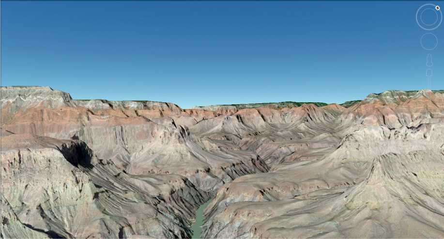   (Source: Google)
5. There are two references to heights or elevation values in the bottom portion of the view:
   • The heading marked “elev” shows the height of the terrain model (that is, the height above the vertical datum) where the cursor is placed.
   • The heading marked “Eye alt” shows Google Earth’s measurement for how high above the terrain (or the vertical datum) your vantage point is.
   
   Maneuver your view so your “Eye alt” is a good level above the terrain, and you’ll be able to see over the mountains and into the canyons—this will be a good height to start flying over the terrain.
6. Use the mouse and the Move tools to practice flying around the Grand Canyon. You can fly over the terrain, dip in and out of valleys, and skim over the mountaintops. When you’ve got a good feel for flying over 3D terrain in Google Earth, move on to the next step.

13.2 Recording Animations in Google Earth

1. On Google Earth’s toolbar, select the Record a Tour button.
   

   (Source: Google)
   
   This option will have Google Earth record your flight and save it as a video. A new set of controls will appear at the bottom of the view:
   
   

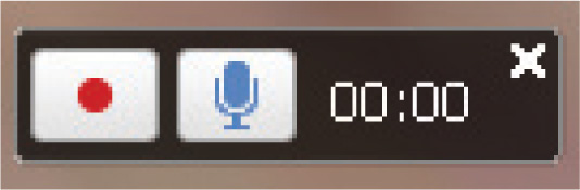   (Source: Google)
2. To start recording the video, press the red record button.
   Important note: If you have a microphone hooked up to your computer, you can get really creative and narrate your flight—your narration or sounds will be saved along with your video.
3. Keep flying around for a short tour (30 to 60 seconds) of the Grand Canyon. Put together a good tour (perhaps about a minute long) of the Grand Canyon that shows off many of the area’s terrain features.
4. When you’re done, press the red record button again to end your recording of the tour.
5. A new set of controls will appear at the bottom of the screen, and Google Earth will begin to play your video.
   

   (Source: Google)
6. Use the rewind and fast-forward buttons to skip around in the video, and also the play/pause button to start or stop. The button with the two arrows will repeat the tour or put it on a loop to keep playing.
7. You can save the tour by pressing the disk icon (Save Tour) button. Give it a name in the dialog box that opens. The saved tour will be added to your Places box (just like all other Google Earth layers).

   Question 13.1

   tBpAuVPhAesi88oxxiItee99ynG5ZrXNT4XinCDHcHFR9/8NlvmRnOhN3NWDrZ0VgrF+13hHx29kBrEvrbRxEJ3krUJxnFWViZvxKoo5nhXHwTICF2qilgwoT4Dwo4aqkVTV7veT/4D6yX8cAXrevxcJtajBkjjyK+vuxfcbaUc=

13.3 Vertical Exaggeration and Measuring Elevation Height Values in Google Earth

Google Earth also allows you to alter the vertical exaggeration of the terrain layer. As we discussed, vertical exaggeration is used for visualization purposes.

1. To look at different levels of vertical exaggeration, select Options from the Tools pull-down menu. Select the 3D View tab.
2. In the box marked Elevation Exaggeration, you can type a value (between 0.01 and 3) for vertical exaggeration of Google Earth’s terrain. Type a value of 2, click Apply and OK, and then re-examine the Grand Canyon.

   Question 13.2

   zXse8KjitA8ZS0if0BRB/G0kVWmeYM15LYs5h4Q8YTKp/sefM3XzwlF5yKpjK7q6iMgPPQQmYnYBjDbCeHg9L7Hj8m/rbzz3VpIVRClgUNhROQfqtWGX5V5MWAmOprYB+r/OXGXV9WhgcJW8fMM0+httO80hgWLt+tNSnTuPajRP2qnDHeWVjHjMVDyO7c2wHeF8icWdo29FmUgo2lYcJ3K2sIwTNKkN3aMQ6Phwpz5KjHGyETcbpJJwLXAPmTv49Tqyu2ztA2i0C5ghLOiexBtRtUYqooEd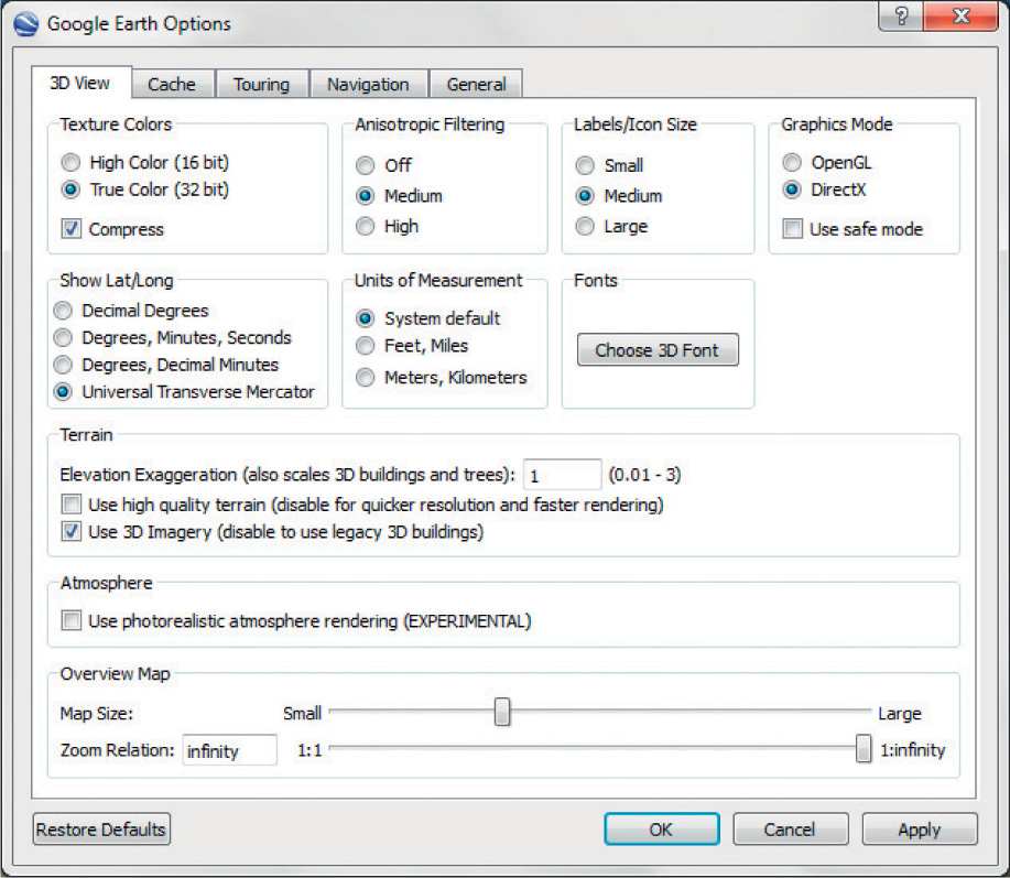
   

   (Source: Google)
3. Reset the Elevation Exaggeration to a value of 1 when you’re done. From here, we’ll examine the elevation values of the terrain surface itself. Although Google Earth will always show the imagery over the terrain model, elevation information of each location is available.
4. In the Layers box, under the More option, turn on the Parks and Recreation layer. Several new symbols will appear around the Grand Canyon, designating specific locales within the park. Wherever you move the cursor on the screen, a new value for elevation is computed in the “elev” option at the bottom of the view. By zooming in to one of the new marker spots and placing the cursor on its symbol on the screen, you can determine the elevation value for that location.

   Question 13.3

   QU+8nrsNvhhMfvUldPEuspSKQot3CvkxIADZtXcj4jYKfIhbpe1oQ/V+gMEM2Lq8xge7U/fbzcXg360NshHeId7IWbW7gPdAvRCsYXMWzZ2ycnpPd+2B82dEdRNzNVmgheRZB1IG86fByUXxwB6wvc311gKBKmml81HabXAzfGK/9CaMACGstLC9tl1vA31xlt1FOH7Zrjo=
5. At this point, we’ll be moving onto a new software package called MICRODEM, which allows you to work directly with both the terrain models and data, not just with the fully processed versions in Google Earth.
   Important note: Don’t close Google Earth just yet. You’ll use it later for another way to take a look at the data you’ll be using next with MICRODEM.
6. Use Google Earth to “Fly To” Hanging Rock Canyon, California.

13.4 Getting Started with MICRODEM

1. Start MICRODEM (the default install is an icon called MICRODEM). It will open with the default screen, full of buttons on the toolbar.
2. To examine a DEM, select the File pull-down menu and choose Open, then choose Open DEM.
3. When MICRODEM installed, it added a new folder called “mapdata” to your computer (the default location is a C:\mapdata folder). Navigate to this folder, select the folder called DEMs, and then select the HangRockCanyon_DEM_2.tar.gz file.
   

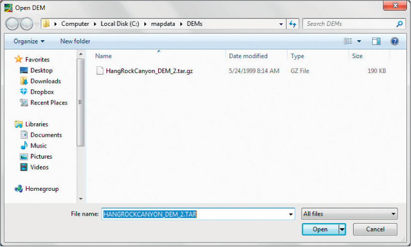   (Source: USNA)
4. Click Open to start using this DEM in MICRODEM. (The DEM will open in a new viewer.)
5. Before moving on, use the DEM and the view in Google Earth to orient yourself to where, spatially, Hanging Rock Canyon is, and what section of the landscape is being displayed by the DEM.
6. When you have yourself oriented, right-click anywhere on the DEM and a new menu will appear. From the available options, select Export, then select Quick map to Google Earth.
7. MICRODEM will then apply a draped image of the DEM over its corresponding area inside of Google Earth (and add a new object called MICRODEM to Google Earth’s Temporary Places folder). This will show you where the DEM’s parameters match up with the Google Earth imagery.

13.5 Hillshades

1. Return to MICRODEM. To change the appearance of the Hanging Rock DEM, right-click anywhere on the DEM, and a new menu will appear. From the available options, select Reflectance Options. You could also select Display parameter, and then choose Reflectance.
2. In the Reflectance Map Options dialog box that opens, select Grays for the Colors option.
3. You’ll also see options for Sun azimuth (default of 335 degrees) and Sun elevation (45 degrees above the surface). The circle in the upper right of the dialog box shows the position of the Sun relative to the DEM with a red dot. This use of the values for azimuth and elevation creates the hillshade effect for viewing the DEM. To create other visualizations of the landscape, you can use other values for Sun azimuth and Sun elevation.
   

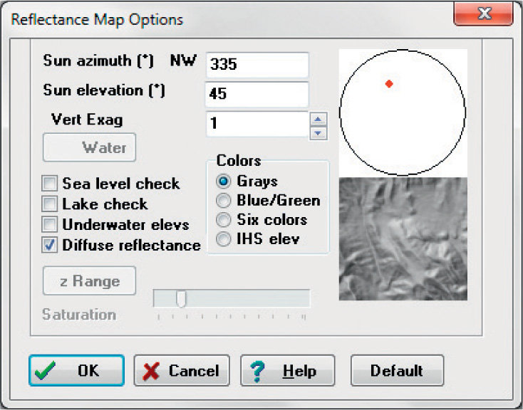   (Source: USNA)
4. Change the Sun azimuth to 90 and the Sun elevation to 10, and then click OK.

   Question 13.4

   6iM0OTYOqcYAH7dSpamkmWKaxE0aMegoPehgH25gxiSOs/kI739PiDtBHneHPlrFECJXIgvkv4oKnQIN8V7vvywmp2WVfAYaFIbpuXTnYmH+v4/nYv6e975gevxi+hqihwS+F87xjCw=
5. Return to the Reflectance Map Options. Test out the effect of other hillshade visualizations based on some other Sun azimuth and Sun elevation values. Answer Question 13.5. When you’re done, return to the norm of Sun azimuth = 335 and Sun elevation of 45.

   Question 13.5

   gaNPITiMZqTwM6ZAwvVavWwJbFrrCT8yYMYQRmykdB/okbdzz5uhy5KKC5p9OsL2LItaoWp6REmE+aJ54vzQdJctdEEoPMar4ao1eefAQoSXFPxuJWRMUoVh5pKSPEERfzoG4m4D9p2BbtSGO7lUVdpb+8Y=

13.6 Contour Lines and Contour Interval on a DEM

1. Contour lines can be generated from the DEM and then displayed as a map overlay (among other layers) to examine how the contours match up with the terrain represented by the DEM. To see the overlay options, select the Manage Overlays icon from the view’s toolbar.
   

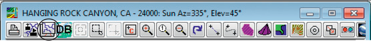   (Source: USNA)
2. In the Map Overlays dialog box, placing a checkmark in one of the options will turn on that particular overlay. Place a checkmark in the Contours box and a new button labeled Contours will be added. Press this button to examine the Contour Intervals.
   

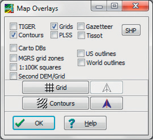   (Source: USNA)
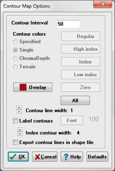
3. In the Contour Map Options dialog box, you can specify the Contour Interval of the contours to be drawn on the DEM.
   

   (Source: USNA)
4. Make sure the Contour Colors option is set to Single.
5. Use 50 meters for the Contour Interval, and then click OK. The contours will be drawn over the DEM.
6. Contours drawn with a 50-meter interval will be placed on the DEM as an overlay. Bring up the Map Overlays dialog box again, press the Contours button, and switch the contour interval to 100 meters. The 50-meter contours will go away and be replaced by new contours drawn at a 100-meter interval.
7. Try out several different contour intervals as follows: 5 meters, 25 meters, 250 meters, and 1 kilometer (in addition to the 50- and 100-meter options). See how the use of those intervals changes the way contours are created and drawn.

   Question 13.6

   Xf2Knwh7Fi6u4uqzpjB04hZ1VBC8PdMayyMki6LS0UIj818yvL2HGxNJwanj5J4yPMT2N+IDprqb+ptAYwAxnYXiSv37Mlowa1Lq+QovimQIdTDBGQLJEUO21xrvX9qUY/nUn3QVtvRQxj6O8RLBlTomBe7kr6HP2DCHjZGYb4c/MErloRkfw3H3PpVU4Wm9vcKN8w3s7iPvgqeex94wCC3Cs+PZMtgtV/tL42qedqhLUU/XUxYxjG9QkyVEVf4FNy5bg2V4n44EMt3gz/ChKIfKkUGMz9lWePYCvyD9PljVbP4jIT+2Gt6EBxTQKluJ58GYVu6PypkKqX1A+P6N3Xp7lNGVZlaP9GAdy2LLEHcP4kqn2UnfA7JyS/Wip8IlNmry3eYkBi4v0dQ307KM0o4CqBaGSs1Y6HRMZSGZRdlJHE2locgVbUeyLqa2eC+lre3e+sTr8zvptLi7gFBuDsuIs6+XnFU8q89r4rhmKB+LMHqGNGucJlZzv7k=

   Question 13.7

   lerb0JWCkPkXReXN0bcZTxPtvA2PwDN7ye+hR8QslnCqYucSCbier/R8kSdg8ZlIJa1KAx6wJc3Yni4K6uknr3dFdWi0dHH0gw5qysJ0xV/fsqSS+4l0a3+951JnnqdMJg5/i1OdaupD1ysKCkHucMPUl/fVVl/CFZiNGVPKxk4DpclMdZLjgMaIRGN2ofIjOWLP5xn5P+GbnmSaDglIdIQ0kQaoL66yoUZYk44wtn/4aImIsqKLLvU0CoIubR1U3zO+xF9pNOYcF/v4sbjTwpzVyL6HQFCmM6UQraPT9zniTk4aFuseFDXbYBsRs78uQXk+SW7y1BDC7pNSI6T9RJSY3LZErUBnxjciF/YWWUu51Gvdevz/48JHfYKuoxx3

13.7 Slope and a DEM

1. Because a DEM is showing elevations, factors such as the slope (for each location) can be derived. Right-click on the DEM, select Display parameter, and choose Slope.
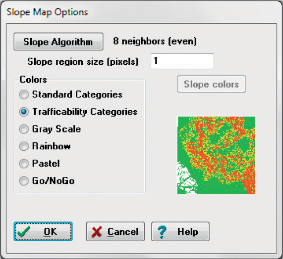
2. In the Slope Map Options dialog box, select the option for Trafficability Categories.
   

   (Source: USNA)
3. Click OK.
4. MICRODEM will calculate a measurement for slope (in degrees) for each location on the DEM.
5. Examine the new slope map.

   Question 13.8

   fwJ8qoWqgN9G/yw7zHZ9ye1Ct29pxSFBCJhXqy/aNXKsvX3HNGFHm2iXJWYefx60GejsMAC9KehnoVAxa3iPXKqaFmz1/QYp/ALD8gvLmj1MaxCoe8eolXYuY9Ufa1XMgt1yrip3T4nAR9XyKcKHT3ZwySfcBVbDvk4+/zUjzcxKmxiP+vtoj1fTikT3P0uw+AjZMgN5ry/fDO9k
6. Re-open the DEM again to place it in a new view.

13.8 Three-Dimensional (3D) Visualization of a DEM

1. The last thing we’re going to do in this lab is examine the DEM in a pseudo-3D view, and do some more flying. In a program like Google Earth, the terrain data has already been processed for you to work with—in these steps, we’re actually going to set up the pseudo-3D view.
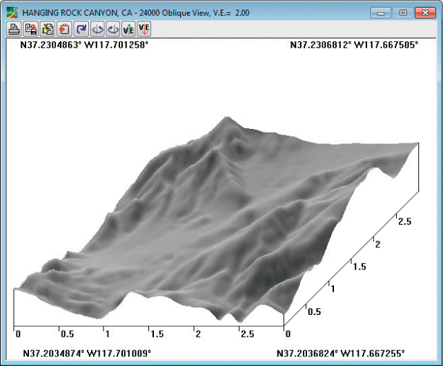
2. From the main MICRODEM toolbar, click on the Oblique View button.
   

   (Source: USNA)
3. The Oblique View will enable you to take a section of the DEM and examine it in oblique perspective view. After clicking on Oblique View, double-click on a section of the DEM and then drag the mouse to another section. The box that you are drawing by double-clicking and dragging represents the area of the DEM that will be shown in perspective view. Double-click again when you’ve set up the box for the area you want.
   Important note: Be sure not to select too large an area. MICRODEM may not be able to handle a section that’s too big.
4. The Oblique View of the DEM section will appear. A new toolbar is part of the Oblique View. The controls will allow you to (in order):
   • Print the image
   • Save the image (as a graphic)
   • Edit the image (in a photo manager program)
   • Copy the image to the clipboard (to use in programs like PowerPoint or Word)
   • Redraw the image with different parameters
   • Rotate the image counterclockwise (to see different sides of it)
   • Rotate the image clockwise
   • Increase the vertical exaggeration
   • Decrease the vertical exaggeration
     

     (Source: USNA)
5. Close the Oblique plot when you’re done investigating it. This tool will allow you to generate a perspective image of a part of the DEM, but in order to interact with the DEM in a pseudo-3D environment, MICRODEM has other tools.
6. In the main MICRODEM toolbar, select the Fly through icon.
   

   (Source: USNA)
7. In the DEM, double-click on a starting point for flying. Drag the mouse in the direction you want to fly, and then double-click the mouse again. A red line will be drawn between the two points. If you want to add a second leg to the flight, drag the line in another direction and double-click again. This red line indicates the flight path—once you have the flight path set up, right-click the mouse and choose End selection.
8. A new dialog box will appear. Select the Viewport tab. These options will allow you to change factors like how high you will be flying over Earth (the Observer above ground option) or the Observer elevation. For your first flight, just accept the defaults and click OK.
9. Two new windows will appear—one showing the flight path as red and black lines, and another showing a video clip of flying over the DEM.
10. MICRODEM will prompt you to “Continue w/these parameters?” Click Yes to watch the video clip.
11. A short clip will play and then a new dialog box will open, prompting you to open a movie. Select the file called FLYT.MOV and click Open.
12. A set of controls will appear at the top of the screen as part of the PETMAR Trilobites Movie Player, to allow you to play, pause, rewind, set up a loop, or alter the delay between the images shown that make up the animated video.
    

    (Source: USNA)
13. You can stop playing and exit the video at any time and return to change flying options, or select a new path to fly over. Play around with some of the flying options, then answer Question 13.9.

    Question 13.9

    ivhc82CgRHiiEH35E8UXmfnEklDGDE91jQhwDSIdsplD8owE7xX/Ud/BSu9GUC+DbN/1VNTLUziYhdJ0JSZYju5Ak+3JDTnOFhXFxdpxFwu/L4SS1NentQHeAz9j4Poir83hQjX5u5HvKX72TaMcUg==

Closing Time

MICRODEM is a very powerful program with a lot of functionality and options for working with DEMs and digital terrain analysis—and it has plenty more features to investigate for your own future use. When you’re finished, close both MICRODEM and Google Earth.