15.1 Geospatial Lab ApplicationExploring ArcGIS Explorer

This chapter’s lab will introduce you to the use of Esri’s free ArcGIS Explorer software program, in the context of many of the concepts introduced throughout the book. In lots of ways you can think of this lab as a “summary” of some of the things you’ve explored in other chapters. However, you’ll be using a new geospatial technology program—ArcGIS Explorer contains numerous GIS tools, as well as access to many different types of GIS and remotely sensed data. You’ll also be using cloud resources available through ArcGIS Explorer in the form of several types of basemaps, data, and imagery.

Objectives

The goals of this lab are:

• to learn the basics of the ArcGIS Explorer environment.
• to utilize various imagery and data sources streamed from the cloud.
• to examine digital topographic maps and understand how terrain is displayed with contours in 3D environments.
• to examine basemap imagery and visually identify features from it.
• to locate an address, create a buffer around it, and calculate a route between two points on a map.

Using Geospatial Technologies

The concepts you’ll be working with in this lab are used in a variety of real-world applications, including:

• engineering, where streaming digital topographic maps are utilized in the planning of new roads or highways in order to examine terrain conditions such as elevation, steepness, and land cover.
• county auditing, where auditors examine streaming high-resolution imagery of residential and commercial properties to assist them in assessing property taxes.

(Source: Mint Images—Tim Pannell/Getty Images)

Obtaining Software

The current version of ArcGIS Explorer Desktop (Build 2500) is available for free download at http://www.esri.com/software/arcgis/explorer/download.

Important note: Software and online resources sometimes change fast. This lab was designed with the most recently available version of the software at the time of writing. However, if the software or Websites have significantly changed between then and now, an updated version of this lab (using the newest versions) is available online at http://www.whfreeman.com/shellito2e.

Lab Data

There is no data to copy in this lab. All data used in this lab comes with the software or is streamed to you via the cloud.

Localizing This Lab

This lab focuses on various features around southern California, but the same techniques can easily be used for a local area. The basemaps used for analysis of Sections 15.2, 15.3, and 15.4 can be adjusted for a local area (as the basemaps cover the whole of the United States). Similarly, the addresses and analysis of Section 15.5 can be performed with local landmarks instead of Hollywood ones.

15.1 Getting Started With ArcGIS Explorer

1. Start ArcGIS Explorer (AGX). You’ll see that it opens with its default satellite imagery of the world (acquired by systems like those described in Chapters 11 and 12).
   
   

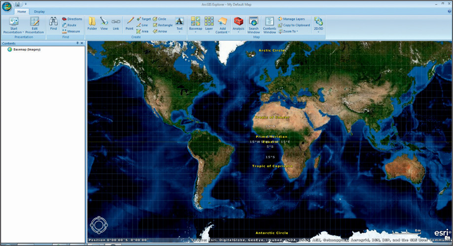   (Source: Esri)
   
   To start things off, you’ll be examining how terrain is modeled and displayed with contour lines on topographic maps (as in Chapter 13). Rather than needing copies of paper topo maps or having to download several quads of digital raster graphics (DRGs) and use them together, ArcGIS Explorer allows you to access an entire set of digital topographic maps (shown at different map scales, depending on what scale you’re working at) via the cloud. These topos are also seamlessly blended into one another, so there are no issues with matching map edges against one another.
2. Select the Find option.
   

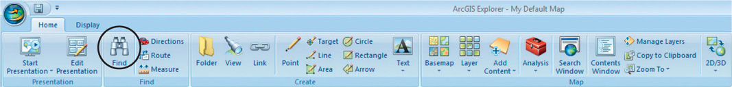   (Source: Esri)
3. We’re going to begin in southern California, just outside of Hollywood. In the AGX Find box, type Tujunga Valley, and click the Search button.
   

   (Source: Esri)
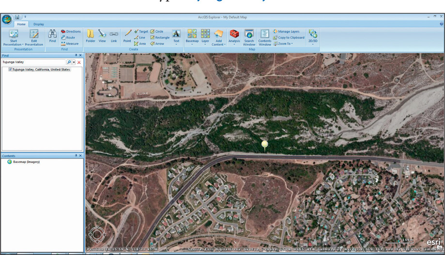
4. An option for Tujunga Valley, California, United States, will appear in the Find box, and AGX will zoom in to the valley in southern California.
5. A pushpin will appear to mark Tujunga Valley on the map. Remove the checkmark from the option in the Find box to remove the pushpin. At this point, you can also close the Find box. Zoom in closer so that you can see the valley.
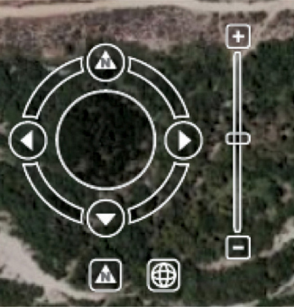
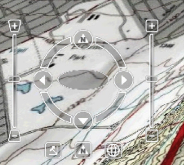
6. A set of controls for navigation in AGX is available in the bottom left-hand corner of the view. Scroll your mouse over that area to enlarge the controls and make them visible. You’ll see that they are similar to Google Earth’s—arrows for navigation and a zoom slider for zooming in and out of a scene. The wheel will spin your view while the “N” button will reset the orientation to the north. You can also use the mouse to pan around, and the mouse wheel to zoom in and out.
   

   (Source: Esri)
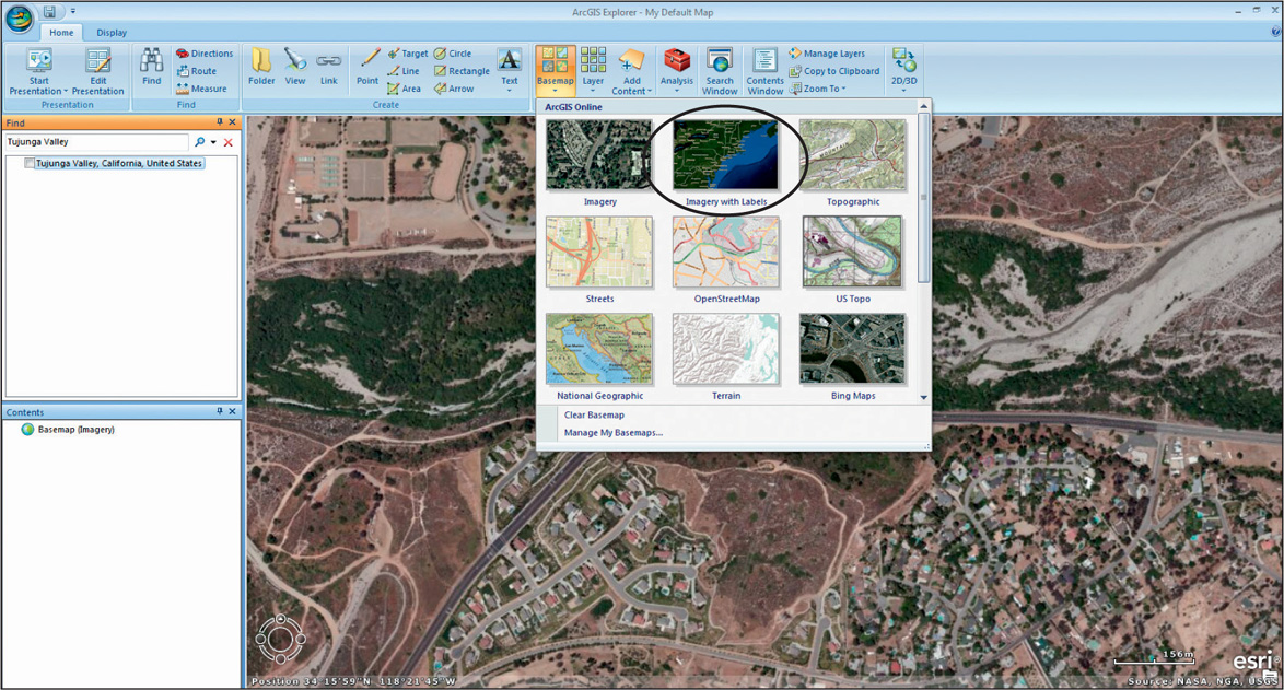
7. To get your bearings in the area with labels on the various cities and features, select the Home tab, and then select the Basemap option. From the new available options, select Imagery with Labels.
8. You’ll see that labels will now start appearing around the map. By zooming in and out of different parts of the image you should be able to make out the cities of San Fernando and Burbank (and Hollywood), with Tujunga Valley separated by two sets of mountains. Zoom in to this region.
   

   (Source: Esri)

15.2 Examining Digital Topographic Maps with ArcGIS Explorer

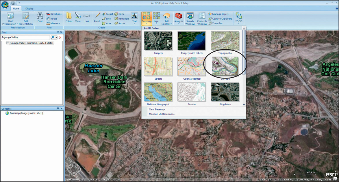
1. To switch to display the topographic maps (that is, to stream them in from the cloud), select the Home tab, and then select the Basemap option. From the available options, select US Topo.
   

   (Source: Esri)
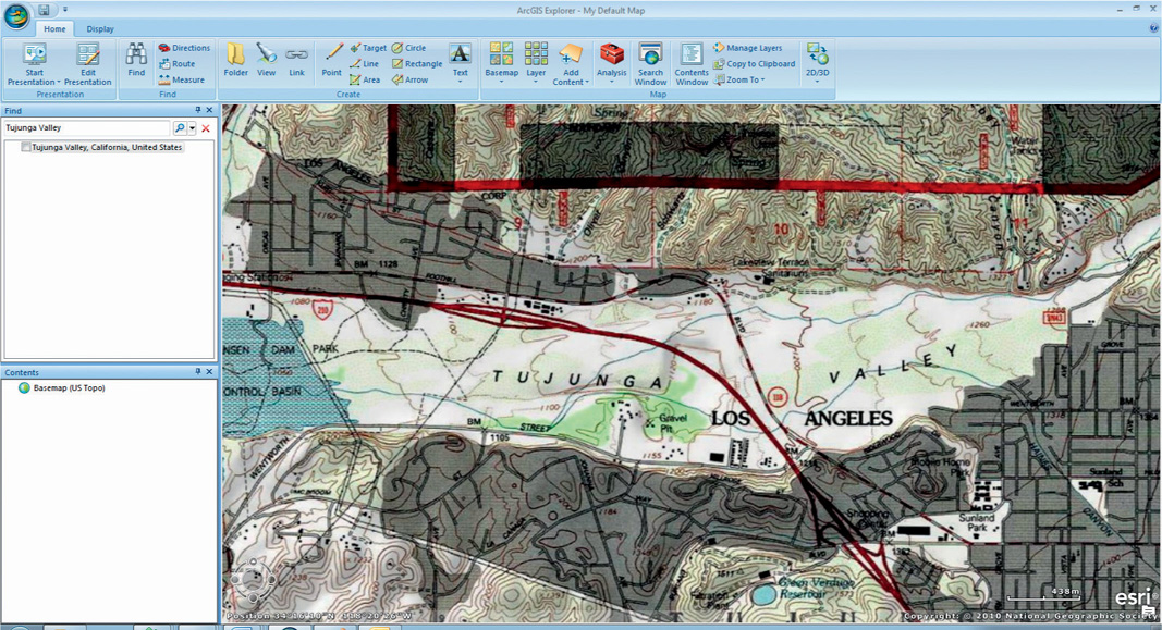
2. AGX will display the digital versions of the USGS topographic maps draped over the terrain. When you’re zoomed out, small-scale digital topos will be displayed, and when you’re zoomed in, AGX will load large-scale digital topos in their place.
3. Zoom in on Tujunga Valley itself, and give AGX a little time to load the larger scale topos for the area.
   

   (Source: Esri)
4. Examine the area around Tujunga Valley (along with the mountains to the north of the valley, and Los Angeles to the south) with respect to the contour lines shown on the map.

   Question 15.1

   How do the contour lines effectively represent the terrain of the valley (as opposed to the mountains)?

   Question 15.2

   From examining the contour lines on the largerscale topographic map that appears once you’ve zoomed in, what is the contour interval of the map?

   Question 15.3

   From examining the contour lines and heights, what are the highest and lowest elevations of Tujunga Valley itself?

15.3 Examining 3D Imagery with ArcGIS Explorer

1. A lot of information about the terrain can be gained from the contours on the topographic maps, but AGX also provides a way to examine imagery in a pseudo-3D way.
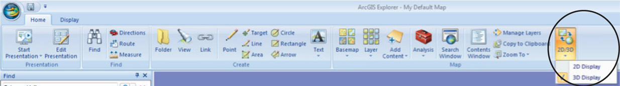
2. To set things up in pseudo-3D, first select the Home tab, and then select the 2D/3D option.
   

   (Source: Esri)
3. Select the option for 3D Display. Give AGX a few seconds to adjust to the 3D view. You’ll now see that a new control has been added to the navigation controls—a second zoom slider has appeared on the left-hand side. This second zoom slider is used to tilt the terrain up and down. You’ll see the disc in the center change perspective as you tilt the terrain.
   

   (Source: Esri)
4. Tilt the view so that you’re looking at the valley (and the surrounding mountains) in perspective view. Pan and zoom around the area—as you do so, you’ll see how the contour lines match with the elevations.
5. Next, switch your basemap to the Streets option.
6. With the Streets Basemap draped over the terrain, you’ll be able to make out details around the valley, and see how the roads wind through the mountains.
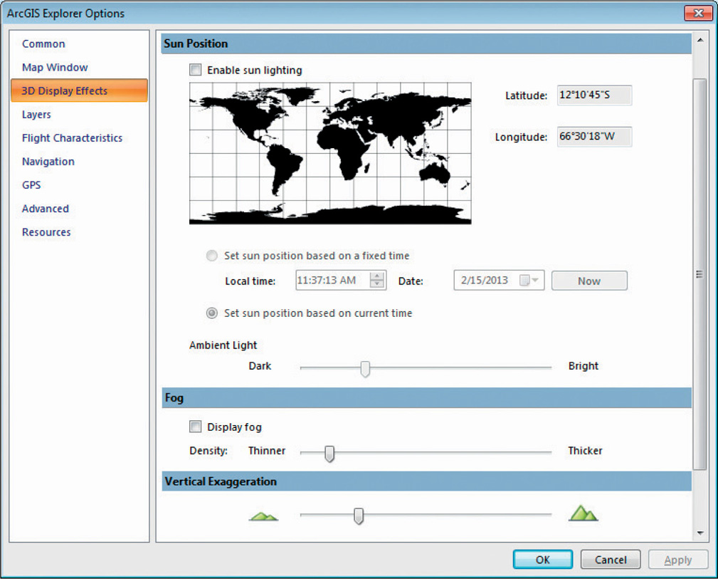
7. Next, you’ll check the terrain’s Vertical Exaggeration. Press the ArcGIS Explorer Button (the icon that has the AGX logo—the globe with the arrows—in the upper left-hand corner of the screen), and then click on ArcGIS Explorer options.
8. In the new window that opens, select the option for 3D Display Effects, and scroll down to Vertical Exaggeration.
   

   (Source: Esri)
9. The Vertical Exaggeration option has a slider bar, with the default setting being the slider at the bottom of the scale (the minimum Vertical Exaggeration). You can change the Vertical Exaggeration all the way up to the maximum (click Apply after each setting). Try a few different settings—at the minimum, then about one-fourth of the way across, then about one-half the way across, then about three-fourths of the way across, and finally at the maximum. At each level, examine how the roads and mountains change appearance.

   Question 15.4

   What were the effects of each level of Vertical Exaggeration? Which would be the best level to use for visually analyzing the area, and why?
10. Reset the Vertical Exaggeration level to about one-fourth of the way up the slider. This level is good for this visualization part of the exercise, as it will really make the mountains and valleys stand out. Even by looking straight down on the streets map, you should be able to discern some illusion of depth in the image (this is from the streets imagery being draped over AGX’s terrain).
11. Use the mouse and controls to fly around the region, zooming and rotating where necessary.

    Question 15.5

    How does viewing draped imagery in perspective help in determining the differences in terrain between Tujunga Valley and the nearby mountains? How does it help in viewing the terrain and landscape features of southern California?
12. Return to the 2D Display when you’re finished.

15.4 Examining High-Resolution Imagery and OpenStreetMap with ArcGIS Explorer

1. Back in Chapter 9, we looked at high-resolution digital imagery—this same kind of imagery is available for AGX via the cloud resources. To view this high-resolution imagery, switch your Basemap over to Imagery.
2. Reposition your view back to Tujunga Valley itself, and carefully look around the region in the valley.

   Question 15.6

   By using the high-resolution imagery and your visual image interpretation elements, what kinds of land uses can you see within Tujunga Valley? For instance, you can make out a highway cutting through the middle of the valley, but what is to the immediate east of the highway? What elements of visual image interpretation help you in discerning what this is?
3. To get more information about various features, you can utilize a different basemap, such as the OpenStreetMap resources (see Chapter 1). Switch your Basemap over to OpenStreetMap.
4. AGX will switch to a new set of data to be streamed to you—not only the images, but labels and other information as well. Examine the new scene of Tujunga Valley, and answer Question 15.7 (this will probably also help confirm your answer to Question 15.6).

   Question 15.7

   What is the name and number of the interstate that goes through the valley?

15.5 Geocoding Addresses and Basic Spatial Analysis with ArcGIS Explorer

1. Back in Chapter 8, we looked at geocoding addresses and routing between them. AGX contains these features, as well as several types of GIS spatial analysis functions. To get started, we’ll begin at a Hollywood landmark: the TCL Chinese Theatre (formerly known as Grauman’s Chinese Theatre—for more information about the theatre, visit http://www.tclchinesetheatres.com).
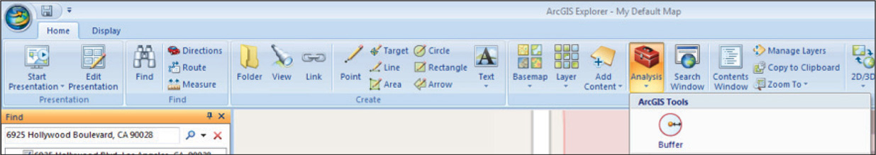
2. Bring up the Find dialog box again (as in Section 15.1), and search for the theater’s address: 6925 Hollywood Boulevard, Hollywood, CA 90028. Click the Search button and AGX will change the view so that it centers on the theater, placing a white pushpin in its location on Hollywood Boulevard. Zoom in closely to the pushpin and you’ll see it placed just outside of the Chinese Theatre (which will be labeled on the OpenStreetMap basemap).
3. You’ll now create a buffer around a point representing the theater (as in Chapter 6). From the Analysis pull-down menu, select Buffer.
   

   (Source: Esri)
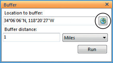
4. In the Buffer dialog box, you can either specify a location (by coordinates) or interactively select a point to create a buffer around. To select a point representing the theater, press the Select button next to the Location to buffer space. The cursor will change to a crosshairs—click on the pushpin marking the TCL Chinese Theatre, and AGX will translate your mouse click into a set of latitude and longitude coordinates representing that point (see Chapter 2 for more about coordinates).
   

   (Source: Esri)
5. Still in the Buffer dialog box, type 1 for the Buffer Distance and select Miles as the units to use, then click Run. AGX will create the buffer. In the Contents Panel, you’ll see a new item added—a one-mile buffer (in red).
6. Zoom out from the theater. You’ll see the circular buffer drawn on the screen, representing a one-mile zone of spatial proximity around the theater.
7. Next, let’s take a look at the location of another Hollywood landmark: the Hollywood Bowl (for more information on the Hollywood Bowl, visit http://www.hollywoodbowl.com). However, we’re going to examine its location in relation to the location of the TCL Chinese Theatre.
8. Select the Home tab, and then click the Directions button.
   

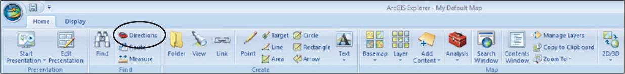   (Source: Esri)
9. In the Directions panel that will open, specify the From Here address as the TCL Chinese Theatre: 6925 Hollywood Boulevard, Hollywood, CA 90028; and then specify the To Here address as the Hollywood Bowl: 2301 North Highland Avenue, Hollywood, CA 90068.
   Important note: You can also interactively select points to use as addresses in a manner similar to picking a point to buffer.
10. Select Miles to Show Distances in and use Fastest as the Route Option. Click Get Directions when you’re ready.
11. AGX will compute the directions between the two places and highlight its chosen “fastest path” in green. Examine the route and the two locations, then answer Questions 15.8, 15.9, and 15.10.

    Question 15.8

    Is the Hollywood Bowl within a one-mile radius of the TCL Chinese Theatre?

    Question 15.9

    What is the driving distance between the TCL Chinese Theatre and the Hollywood Bowl?

    Question 15.10

    Without transcribing directions, what is the “fastest route” to go from one location to the other?

Closing Time

AGX has a lot of other features beyond these, including several other tools, and other types of basemap data and imagery that you can stream from the cloud. Additionally, other geospatial data sources like rasters, shapefiles, and geodatabases (see Chapter 5), KMZ files (see Chapter 14), and GPS data (see Chapter 4) can be added as separate GIS layers.

At this point you can exit AGX by selecting Exit ArcGIS Explorer from the options found by pressing the Explorer button in the upper left-hand corner of AGX, and say good-bye to labs for the rest of the book.