5.2 Geospatial Lab Application: GIS Introduction: ArcGIS Version

This chapter’s lab will introduce you to some of the basic features of GIS. You will be using one of Esri’s GIS programs to navigate a GIS environment and begin working with geospatial data. The labs in Chapters 6, 7, and 8 will utilize several more GIS features; the aim of this chapter’s lab is to familiarize you with the basic functions of the software. The previous Geospatial Lab Application 5.1: GIS Introduction: QGIS Version asked you to use the free Quantum GIS (QGIS) software; however, this lab provides the same activities but asks you to use ArcGIS 10.1 or 10.2.

Objectives

The goals for you to take away from this lab are:

• to familiarize yourself with the ArcGIS software environment, including basic navigation and tool use with both ArcMap and Catalog.
• to examine characteristics of geospatial data, such as their coordinate system, datum, and projection information.
• to familiarize yourself with adding data and manipulating data layer properties, including changing the symbology and appearance of Esri data.
• to familiarize yourself with data attribute tables in ArcGIS.
• to make measurements between objects in ArcGIS.

Obtaining Software

The current version of ArcGIS is not freely available for use. However, instructors affiliated with schools that have a campus-wide software license may request a 1-year student version of the software online at http://www.esri.com/industries/apps/education/offers/promo/index.cfm.

Important note: Software and online resources sometimes change fast. This lab was designed with the most recently available version of the software at the time of writing. However, if the software or Websites have significantly changed between then and now, an updated version of this lab (using the newest versions) is available online at http://www.whfreeman.com/shellito2e.

Using Geospatial Technologies

The concepts you’ll be working with in this lab are used in a variety of real-world applications, including:

• public works, where GIS is used for mapping infrastructure and things such as sewer lines, water mains, and street light locations.
• archeology, where GIS is used for mapping boundaries and the spatial characteristics of dig sites, as well as the locations of artifacts found there.

(Source: Kenneth Garrett/National Geographic/Getty Images)

Lab Data

Copy the folder Chapter5—it contains a folder called “usa,” in which you’ll find several shapefiles that you’ll be using in this lab. This data comes courtesy of Esri and was formerly distributed as part of their free educational GIS software package ArcExplorer Java Edition for Educators (AEJEE).

Localizing This Lab

The dataset used in this lab is Esri sample data for the entire United States. However, starting in Section 5.6, the lab focuses on Ohio and the locations of some Ohio cities. With the sample data covering the state boundaries and city locations for the whole United States, it’s easy enough to select your city (or cities nearby) and perform the same measurements and analysis using those cities more local to you than ones in northeast Ohio.

5.1 An Introduction to ArcMap

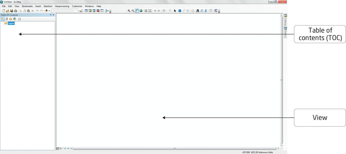
1. Start ArcMap (the default install folder is called ArcGIS). ArcMap will begin by asking you questions about “maps.” In ArcMap, a “map document” is the means of saving your work—since you’re just starting, click on Cancel in the Getting Started dialog box. The left-hand column (where you’ll see the word Layers) is referred to as the Table of Contents (TOC)—it’s where you’ll have a list of available data layers. The blank screen that takes up most of the interface is the View, where data will be displayed.
   
   

   (Source: Esri)
   
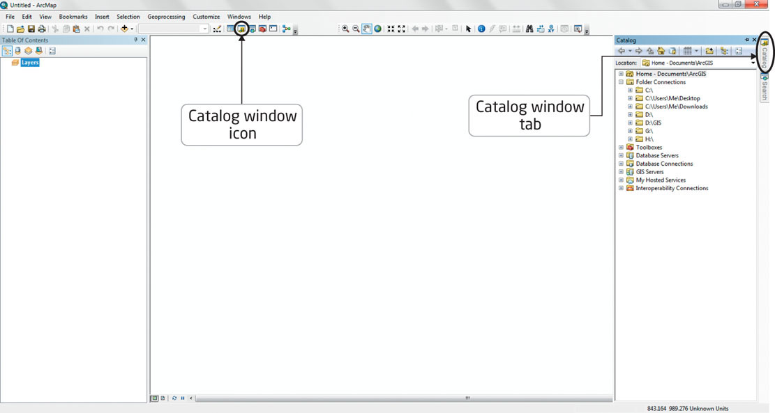
   Before you begin adding and viewing data, the first thing to do is examine the data you have available to you. To examine data layers, you can use the Catalog window in ArcMap—a utility designed to allow you to organize and manage GIS data.
   Important note: ArcGIS 10.1 and 10.2 also contain a separate application called ArcCatalog that can be used to perform the same data management tasks. However, ArcGIS 10.1 and 10.2 incorporate the same functionality into ArcMap’s Catalog window, so you’ll be using that in this Lab, rather than a separate program.
2. By default, the Catalog window is “pinned” to the right-hand side of ArcMap’s screen as a tab. Clicking on the tab will expand the Catalog window. You can also open the Catalog window by clicking on its icon on the main toolbar.
   
   

   (Source: Esri)
   
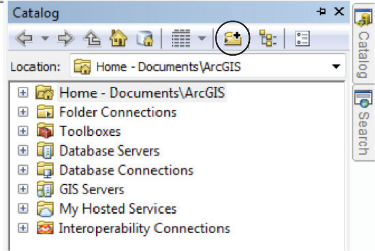
   Important note: Various folders (representing network locations, hard drives on a computer, or external USB drives) can be accessed by using the Connect to Folder button. For instance, this lab assumes the Esri data you’re using in this lab is stored in a folder on the C: drive of your computer.
3. Press the Connect to Folder button on the Catalog’s toolbar.
   

   (Source: Esri)
4. In the Connect to Folder dialog box, choose your computer’s C: drive (or the drive or folder where the lab data is stored) from the available options and click OK.
5. Back in the Catalog, whichever folder you chose (such as C:) will become available by expanding the Folder Connections option.
   Important note: This lab assumes the lab data is stored on the C:\Chapter5\ path. Navigate to that folder (or its equivalent on your computer) and open the usa folder. Several layers will be available, including cities, lakes, and states).
6. The Catalog can be used to preview each of your available data layers as well as manage them. To see a preview of the layers you’ll be using in this lab, do the following:
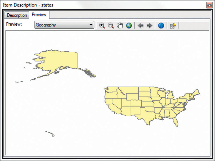
   1. Right-click on one of the layers in the Catalog (for instance, states).
   2. Select the option for Item Description.
   3. A new window will open (called “Item Description – states”). Click on the Preview tab in this window to see what the dataset looks like. Tools will be available in the window to zoom in and out (the magnifying glasses), pan around the data (the hand), or return to the full extent of the dataset (the globe).

(Source: Esri)

Preview each of the shapefiles (selecting a layer’s Item Description will put it into the new window). Note that once the Item Description window is open (and the Preview of the Geography option is selected), you can click once on the name of the file in the Catalog and it will display a preview of that file in the Item Description window.

5.2 Adding Data to ArcMap and Working with the TOC

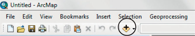
1. Back in the main window of ArcMap, click on the yellow and black “plus” button to start adding the data you’ve previewed in the Catalog to the map.
   
   

   (Source: Esri)
2. In the Add Data dialog box, navigate to the Chapter5 folder, then the usa folder, and select the states.shp shapefile. Click Add (or double-click on the name of the shapefile).
3. You’ll now see the states shapefile in the TOC and its content will be displayed in the View.
4. In the TOC, you’ll see a checkmark in the box next to the states shapefile. When the checkmark is displayed, the layer will be shown in the View, and when the checkmark is removed (by clicking on it) the layer will not be displayed.
5. Now add two more layers: cities (a point layer), and intrstat (a line layer). All three of your layers will now be in the TOC.
6. You can manipulate the “drawing order” of items in the TOC by grabbing a layer with the mouse and moving it up or down in the TOC. Whatever layer is at the bottom is drawn first, and the layers above it in the TOC are drawn on top of it. Thus, if you move the states layer to the top of the TOC, the other layers will not be visible in the View because the states’ polygons are being drawn over them.

5.3 Symbology of Features in ArcMap

1. You’ll also notice that the symbology generated for each of the three objects is simple—points, lines, and polygons, each one assigned a random color. You can significantly alter the appearance of the objects in the View if you want to customize your maps.
   
   

   (Source: Esri)
2. Right-click on the states layer and select Properties.
3. Select the tab for Symbology.
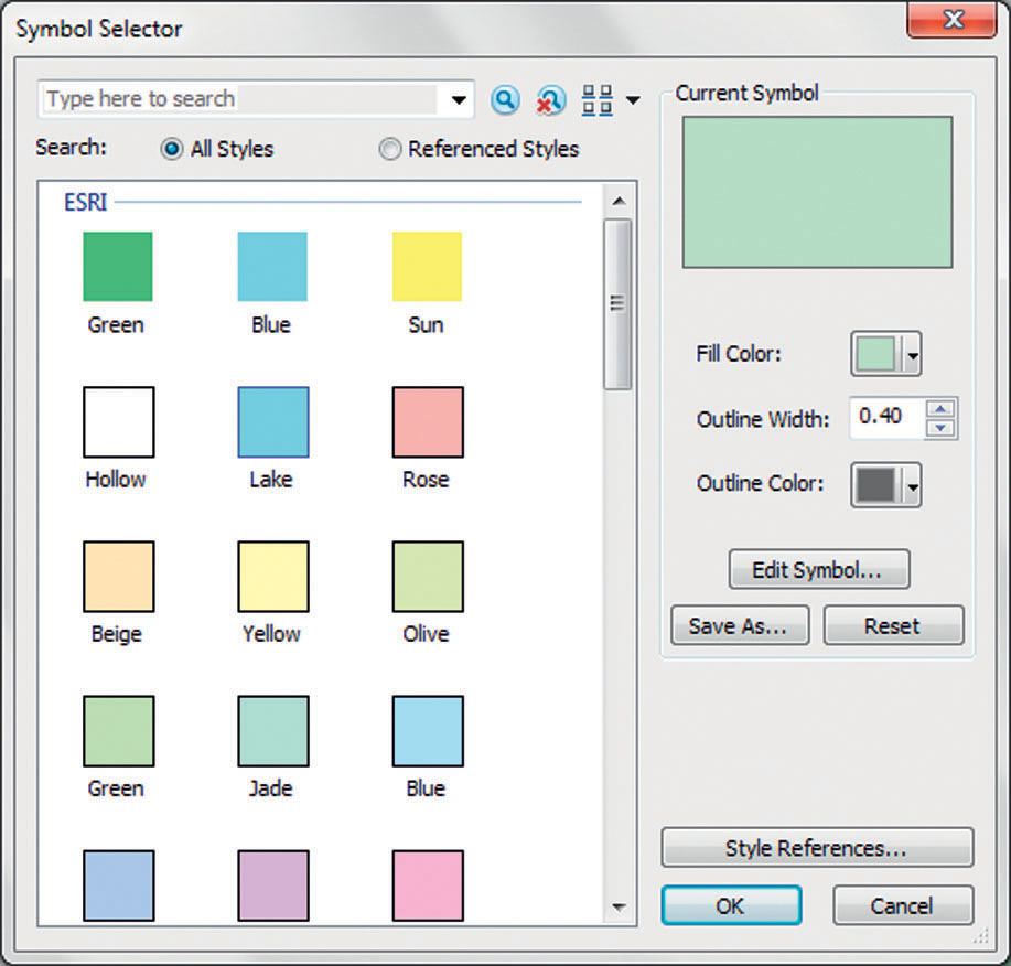
4. Press the large colored rectangle in the Symbol box—in the new Symbol Selector dialog box, you can alter the appearance of the states by changing their color (choose one of the defaults or select from the Fill Color options), as well as the outline color and thickness of the outline itself.
5. Change the states dataset to something more appealing to you, and then click OK. In the Layer Properties dialog box, click Apply to make the changes, then OK to close the dialog. Do the same for the cities and interstates shapefiles. Note that you can alter the points for the cities into shapes like stars, triangles, or crosses, and change their size as well. Several different styles are available for the lines of the interstates file as well.

5.4 Obtaining Projection Information

1. Chapter 2 discussed the importance of projections, coordinate systems, and datums, and all of the information associated with these concepts can be accessed using ArcMap.
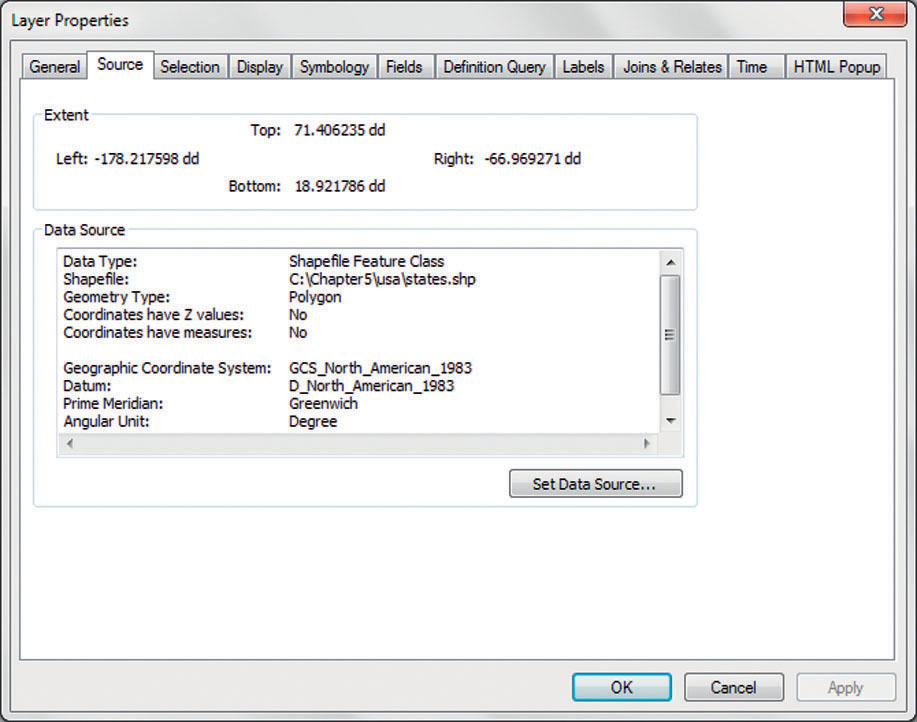
2. Right-click on the states shapefile and select Properties. Click on the Source tab in the dialog box.
3. Information about units, projections, coordinate systems, and datums can all be accessed for each layer.
4. Click OK to exit the states Layer Properties dialog box.
   

   (Source: Esri)

   Question 5.12

   0V+zaTIYaZNSu7M/5Kdg+dMFONWEfreQFtIY8dXfgEQXeZeRCOMZLHYCOut7jbPZar47AGrwvoTaxTS7KXiIpbs0mfCZ4/LhrrMvFb4p9+cSOFgYvGw1Frhcv83QXk1hG3mjyrLO9XBYwlZuX8S3tIRka/Bt0nYi1bdGsmhWsyE8/jOZoMhbYA==

   Question 5.13

   Wl8hqnxHM71PeifjVDBsjJuHptTx2VvdlDFjfQejR9yFC6GMZgRp6kf5PPEbsNmBkz3dUpEgi+TKibeX4Mz4/S6zCug=
   Important note: ArcMap also allows you to change the projected appearance of the data in the View from one projected system to another. In ArcMap, all of the layers that are part of the View are held within a Data Frame—the default name for a Data Frame is “Layers,” which you can see at the top of the TOC. By altering the properties of the Data Frame, you can change the appearance of layers in the View. Note that this does not alter the actual projection of the layers themselves, simply how you’re seeing them displayed.
   

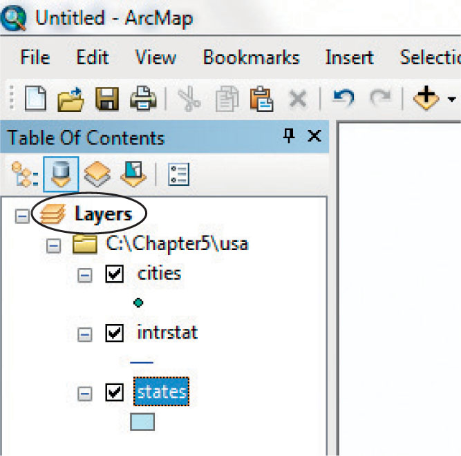   (Source: Esri)
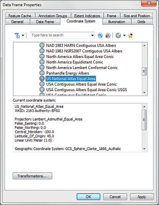
5. Right-click on the Data Frame in the TOC (the “Layers” icon) and select Properties.
6. In the Data Frame Properties dialog box, select the Coordinate System tab.
7. From the available options, select Projected Coordinate Systems, then Continental, and then North America. Lastly, choose US National Atlas Equal Area.
   

   (Source: Esri)

   Question 5.14

   Ga5oDxGIB7XLIZXcGsiK9SXzsC8sHlqQgd0NG/AB/u1XMrqE/xe4nHeSEbhUJWEgnekGVdcr8WrC/kETjehJx9LJvMwMU5l5M8YycHY0eDdxwIURBp5/2Q==
8. Click Apply to make the changes, and then click OK to close the dialog box.
9. Back in the View, you’ll see that the appearance of the three layers has completely changed from the flat GCS projection to the curved US National Atlas Equal Area projection. You can select other projections for the Data Frame if you wish. Try out some other appearances—when you’re done, return to the US National Atlas Equal Area projection for the remainder of the Lab.

5.5 Navigating the View

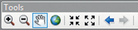
1. ArcMap provides a number of tools for navigating around the data layers in the View. By default, these items are on a separate toolbar docked under the pull-down menus. ArcMap has a variety of separate toolbars to access—the one with the main navigation tools is simply called “Tools.” If it is not present, select the Customize pull-down menu, select Toolbars, and then select Tools from the available choices.
   
   

   (Source: Esri)
   
   Important note: The magnifying glass icons allow you to zoom in (the plus icon) or out (the minus icon). You can zoom by clicking in the window or clicking and dragging a box around the area you want to zoom into.
2. The hand icon is the Pan tool that allows you to “grab” the View by clicking on it, and to drag the map around the screen for navigation.
3. The globe icon will zoom the View to the extent of all the layers. It’s good to use if you’ve zoomed too far in or out in the View or need to restart.
4. The four pointing arrows allow you to zoom in (arrows pointing inward) or zoom out (arrows pointing outward) from the center of the View.
5. The blue arrows allow you to step back or forward from the last set of zooms you’ve made.
6. Use the Zoom and Pan tools to center the View on Ohio so that you’re able to see the entirety of the state and its cities and roads.

5.6 Interactively Obtaining Information

1. Even with the View centered on Ohio, there are an awful lot of point symbols there, representing the cities. We’re going to want to identify and use only a couple of them. ArcMap has a searching tool that allows you to locate specific objects—on the toolbar, select the Find tool (the binoculars icon):
   
   

   (Source: Esri)
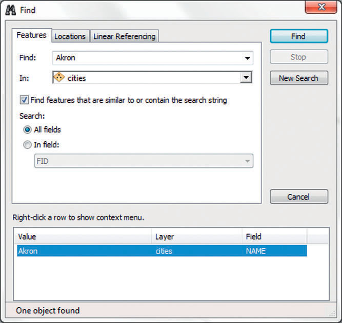
2. In the Find dialog box, select the Features tab. In the Find field type Akron.
   
   

   (Source: Esri)
3. Choose Cities for the Layers to look in.
4. Select the option for All fields for the Search.
5. Click the Find button. The returned results will be shown in the bottom of the dialog box.
6. Drag the dialog box out of the way so that you can see both it and the View at the same time.
7. Double-click on the result for Akron in the bottom of the dialog box.
8. You’ll see that the point symbol for the city of Akron briefly highlights and changes color.
9. Right-click on the same results in the Find dialog box and choose Select from the available options. You’ll see that the point representing Akron has changed color to a light blue. This means it has been “selected” by ArcMap—any actions performed on the cities layer will affect the selected items, but not all of the cities.
10. All that Find can do is locate and select an object. To obtain information about it, you can use the Identify tool (the icon on the toolbar is the white “i” in a blue circle).
    
    

    (Source: Esri)
11. Select the Identify tool, and then click on Akron (zooming in as necessary). A new dialog box will open, listing all of the attribute information associated with Akron (it’s actually giving you all of the field attribute information that goes along with that particular record).
12. In the Find dialog box, right-click on the results and choose Unselect to remove Akron from selection (this will prevent it from being used in the analysis for the next sections).
13. Return to Find and look for a city called Youngstown, then use the Identify tool on the selected city.
    

    Question 5.15

    ePlfy8GDlAuxGuLQ46T3ly18YH6TeXTp5T4cfv2UY6kVtAlj9H0WXjPGLJXkqwMpoh9DskBBkNIsVe+UgYZLpr4wDnd3BiGPbjZXuCbdyLn/6CgZekXQS6aSTkYKcsw+iAQk3ekXyui5exSj/+IejPMb9jGhEjzXaPwfEneKHYUhgONiznb0OVRRBsM=
14. Another method of selecting features interactively is to use the Select Features tool. To select features from the cities layer, click on this icon on the toolbar—a cursor with a white and cyan polygon to its right.
    
    

    (Source: Esri)
15. The Select Features tool allows you to select several objects at once by defining the shape you want to use to select them with: rectangle, polygon, lasso, circle, or line. For now, choose rectangle or polygon, and select the four cities to the immediate northwest and west of Youngstown (note that this will also select features from other layers, although we will just be working with cities in this lab).

5.7 Examining Attribute Tables

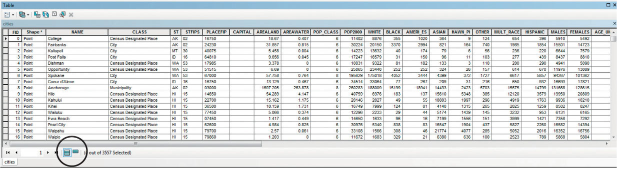
1. Each of the layers has an accompanying attribute table. To open a layer’s attribute table, right-click on the layer in the TOC, then select Open Attribute Table. Open the attribute table for cities.
2. At the bottom of the cities’ attribute table you’ll see that four records have been selected (the four cities nearby Youngstown to its west and northwest). That’s all well and good, but you’ll also see that there are 3557 records in the entire attribute table (which means there are 3557 point objects in the cities data layer). To find those four records would mean a lot of digging through the data. However, ArcMap has some helpful sorting features, including one that will sort through the table and show only the selected records.
3. At the bottom of the attribute table, select the icon for Show Selected Records (it’s the short stack icon in light blue).
   
   

   (Source: Esri)
   
   The four selected records will be highlighted in cyan and these will be the only records shown in the table.
   

   Question 5.16

   XUvNlCjvfOM4lHEXET4Rx8nB4i8bBrL5UUDCtMXqqLR46TPT9Sc2zrpSBvkGwi8Kp12FYAI96A6Axr99WLDQSw==

   Question 5.17

   w/n8MyDwPIHnB3UjHgUwKTh1DHa7m7m0ntNwOMXp6AdU7LL5//RnmILhesxq2SOxLdpORSCH6lpqJWMCpngbo+D2wsm9PtCQywFTiQpDrBYuvirA+mSmK73NeYzuyMLgchC4I42Jf0o0OsQB7P/P+IYCkQU=
4. Close the attribute table. To clear the selected features, select the clear icon on the toolbar (the Clear Selected Features) tool.
   
   

   (Source: Esri)

5.8 Labeling Features

1. Rather than dealing with several points on a map and trying to remember which city is which, it’s easier to simply label each city so that its name appears in the View. ArcMap gives you the ability to do this by creating a label for each record and allowing you to choose the field with which to create the label.
2. Right-click on the cities layer in the TOC and select Label Features. Default labels for the names of the cities will appear next to the points.
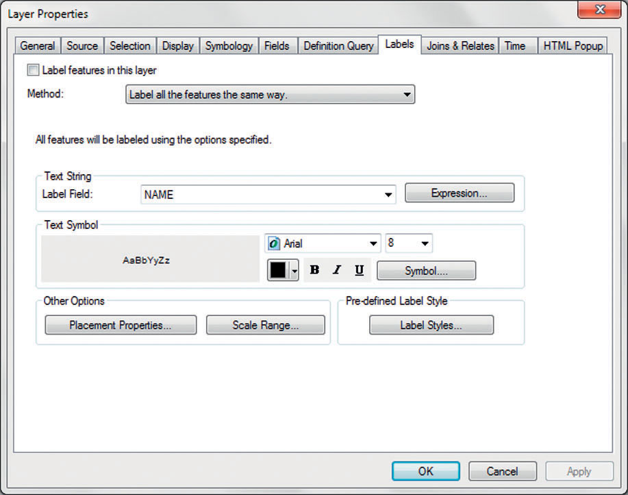
3. To change the appearance of the labels, right-click on the cities layer and select Properties. In the Properties dialog box, choose the Labels tab.
4. Change around any of the options—font, color, text size, (plus options like bold, italics, or underlining), and even the placement of the labels—however you feel is best for examining the map data.
   
   

   (Source: Esri)

5.9 Measurements on a Map

1. With all the cities now labeled, it’s easier to keep track of all of them. With this in mind, your next task is to make a series of measurements between points to see what the Euclidian (straight line) distance is between cities in northeast Ohio.
2. Zoom in tightly so that your View contains the cities of Youngstown and Warren, and the other cities between them.
3. Select the Measure tool from the toolbar—it’s the one that resembles a ruler with two blue arrows over it.
   
   

   (Source: Esri)
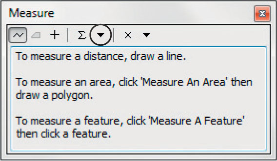
4. In the Measure dialog box, select the Choose Units pull-down menu, then select Distance, and then select Miles (this will return all measurements to you in miles rather than the default of meters).
   
   

   (Source: Esri)
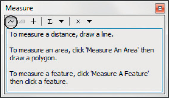
5. Select the Measure Line tool from the toolbar. You’ll see that the cursor has turned into crosshairs framed by a ruler.
   
   

   (Source: Esri)
6. Place the crosshairs on the point representing Youngstown and left-click the mouse (you’ll also see a circle appear around Youngstown). Drag the crosshairs north and west to the point representing Girard (once you’ve reached the point representing Girard, a circle will appear around that point) and left-click the mouse again. The distance measurement will appear in a box in the Measure dialog box. The value for Segment is the planar distance measured on the map for one leg of the measure, while Length is the value for all segments being measured.
7. Continue by measuring another line from Girard to Niles.
   

   Question 5.18

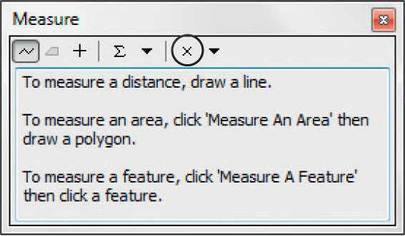
   n8qSvidGu4VqeuMzbZwW/wIznNCVWCEPcSoHKPBAyZ1X1Sk8is5vLk25nCQ/7oXn6gGHAsY2hibsUuoAiatIt1cVfWmg6DMDBjQPjJ+c17LUHmQINF+d7+9V7vI9g/X5kEy9p3HiNm9hWAsmF+KWZzpNlT34Nf+OH7uIPgdd+PI1p1oS
8. Double-clicking the mouse will stop the measurement tool and remove the lines from the screen. To clear the results shown in the measurement dialog box, select the Clear and Reset Results button in the Measure dialog.
   
   

   (Source: Esri)
9. There are a few more measurements to make before you complete this chapter’s questions.

   Question 5.19

   HOJDKYNeSxB+IHiJ8gplo7S0aP+0aXb8gs24nnza1M6xleN/l9kBqF3lANkbD7r6lV8KS8AUGhokIlDX7i8TF0V9011r8YVQU3jokvL7imdOERWdZ8hpbeaGbSI=

   Question 5.20

   XC5On8N+xk79y5AOQCQG5TsE0r1c+r+TFDopaSjJ0wSUaDrOYWPgLGi+8aQLJahI2BR5IWRhOlhMlmIRvWl4Zy6C+pqLn50FyoxmRABaCLHMsMdfgGL71f8Pj4e+1VCDRUi6e+Gd02y2+0zisVpBNWQvZ3+E6v3cM0kfp9Xhm3vD8IUFInKEgfAu394=

5.10: Saving Your Work (and Working on It Later)

When you’ve been using ArcMap, you can save your work at any time and return to it. When work is saved in ArcMap, a map document file is written to disk. Later, you can re-open this file to pick up your work where you left off.

1. Saving to an ArcMap document file is done by clicking on the Save icon on the toolbar (the floppy disk icon) or by choosing Save from the File pull-down menu.
2. Files can be re-opened by choosing the Open icon on the toolbar (the folder icon) or by choosing Open from the File pull-down menu.
3. Exit ArcMap by selecting Exit from the File pull-down menu. There’s no need to save any data in this lab.

Closing Time

This lab was pretty basic, but it served to introduce you to how ArcGIS operates and how GIS data can be examined and manipulated. You’ll be using either QGIS or ArcGIS in the next three chapter labs, so the goal of this lab was to get the fundamentals of the software down. The lab in Chapter 6 takes this GIS data and starts to do spatial analysis with it, while the lab in Chapter 7 will have you starting to make print-quality maps from the data. Chapter 8’s lab will involve some further GIS analysis, this time concerned with road networks.