5.3 How Is Non-Spatial Data Handled by GIS?
attributes the non-spatial data that can be associated with a spatial location
Whether you’re mapping schools ranked by average SAT scores or the locations of the United States’ top tourist destinations, all of this numeric data needs somehow to be represented in GIS. For instance (going back to the digitizing example), if you have two data layers (one containing polygons representing housing footprints and one containing lines representing the driveways), each would contain multiple objects. The GIS will have information about the spatial properties of the objects in that layer, but what it does not have is any other information about those objects (such as the tax-assessed value of the house, the house’s address, the name of the owner, the number of people living in the house, the material the driveway’s made of, or how old the driveway is). All of these attributes represent other non-spatial information associated with each of the objects. When representing attribute data in GIS, these values can take one of four forms: nominal, ordinal, interval, or ratio data.
nominal data a type of data that is a unique identifier of some kind. If numerical, the differences between numbers are not significant
Nominal data are values that represent some sort of unique identifier. Your Social Security number or telephone number would both be examples of nominal data—both of these values are unique to you. Names or descriptive information that are associated with a location would be nominal data, as they’re unique values, the same as a value from a land cover classification scheme. Also, the difference between numerical nominal values is not significant—you can’t add your Social Security number to a friend’s number and come up with a relative’s number—in the same way you can’t subtract your phone number from one friend’s number and come up with another friend’s phone number.
120
ordinal data a type of data that refers solely to a ranking of some kind
Ordinal data is used to represent a ranking system of data. If you have data that is placed in a hierarchy where one item is first, another is second, and another is third, that data is considered ordinal. For instance, if you have a map of the city and you’re going to identify the locations of the homes of the the most successful competitors in a local car-racing event, the points on the map will be tagged as to the location of the first-place winner, the second-place winner, etc. Ordinal data deals solely with the rankings themselves, not with the numbers associated with these ranks. For instance, the only values mapped for the car-race winners is their placement in the race, not their winning times or the cars’ speeds, or any other values. The only thing ordinal data represents is a clear value of what item is first, which is second, and so on. No measurements can be made of how much better the winning driver’s time was than the time of the driver who took second place, only that one driver was first and one driver was second.
interval data a type of numerical data in which the difference between numbers is significant, but there is no fixed non-arbitrary zero point associated with the data
Interval data is used when the difference between numbers is significant, but there is no fixed zero point. With interval data, the value of zero is just another number used on the scale. For instance, temperature measured in degrees Celsius would be considered interval data since values can fall below zero, and the value of zero only represents the freezing point of water, not the bottom of the Celsius temperature scale. However, since there is no fixed zero point, we can make differences between values (for instance, if it was 15 degrees yesterday and 30 degrees today, we can say it was 15 degrees warmer), but dividing numbers wouldn’t work (since a temperature of 30 degrees is not twice as warm as a temperature of 15 degrees).
ratio data a type of numerical data in which the difference between numbers is significant, but there is a fixed non-arbitrary zero point associated with the data
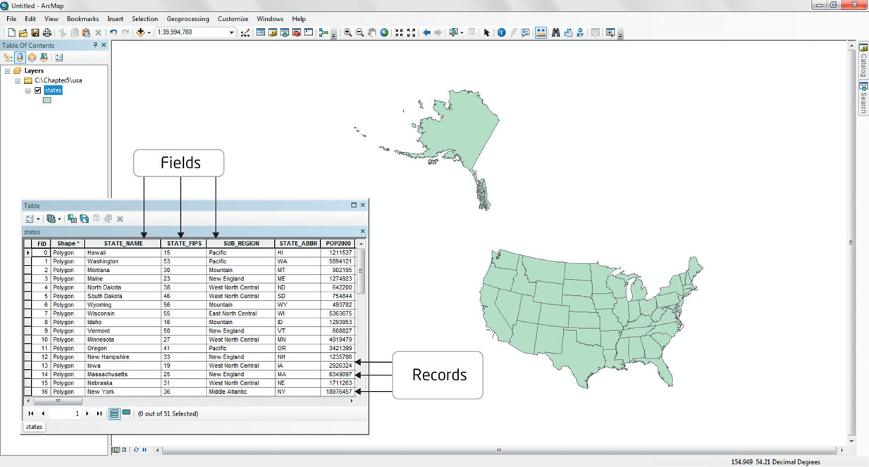
attribute table a spreadsheet-style form where the rows consist of individual objects and the columns are the attributes associated with those objects
records the rows of an attribute table
fields the columns of an attribute table
Ratio data are values with a fixed and non-arbitrary zero point. For instance, a person’s age or weight would be considered ratio data since a person cannot be less than zero years in age or weigh less than zero pounds. With ratio data, the values can be meaningfully divided and subtracted. If we want to know how much time separated the car-racing winners, we could subtract the winning driver’s time from the second-place driver’s time and get the necessary data. Similarly, a textbook that costs $100 is twice as expensive as a textbook that costs $50 (as we divide one number by the other). Ratio data is used when comparing multiple sets of numbers and looking for distinctions between them. For instance, when mapping the locations of car wash centers, the data associated with the location is the number of cars that use the service. By comparing the values, we can see how much one car wash outsells the others, or calculate the profit generated by each location.
Each layer in the GIS has an associated attribute table that stores additional information about the features making up that layer. The attribute table is like a spreadsheet where each object is stored as a record (a row) and the information associated with the records—the attributes—is stored as fields (columns). See Figure 5.8 for an example of an attribute table in conjunction with its GIS objects. To use the housing example again, the houses’ attribute table would consists of five records, each representing a house polygon. New fields could be created, having headings such as “Owner” and “Appraised Value” so that this type of descriptive, non-spatial data could be added for each of the records. These new attributes can be one of the four data types (for instance, “Owner” would be nominal data, while “Appraised Value” would be ratio data). In this way, non-spatial data is associated with a spatial location.
121
A raster attribute table can’t be handled the same way as one for vector objects since a raster dataset is composed of multiple grid cells (for instance, a 30-meter resolution grid of a single county could take millions of cells to model). Rather than having separate records for each grid cell, raster data will often be set up in a table with each record featuring the value for a raster cell and an attribute showing the count of how many cells comprise the dataset. For instance, a county-land-use dataset may contain millions of cells, but only consist of seven values. Thus, the raster would have seven records (one for each value) and another field whose value would be a summation of how many cells have that value. New attributes would be defined by the raster values (for instance, the type of land use that value represents).
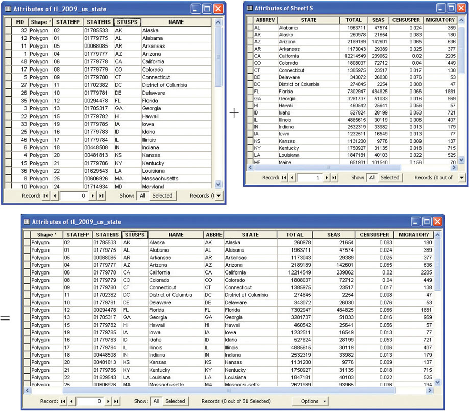
join a method of linking two (or more) tables together
key the field that two tables have to have in common with each other in order for the tables to be joined
Besides creating new fields and populating them with attributes by hand, a join is another way GIS allows non-spatial data to be connected to spatial locations. This works by linking the information for records in one table to its corresponding records in another table. This operation is managed by both tables having a field in common (this field is also referred to as a key). For instance, Figure 5.9 shows two tables, the first from a shapefile’s attribute table that has geospatial information about a set of points representing the states of the United States, while the second table has non-spatial Census information about housing stock for those states. Since both tables have a common field (that is, the state’s abbreviation), a join can be performed on the basis of that key.
122
After the join, the non-spatial Census information from the second table will be associated with the geospatial information from the states’ table. For instance, you can now select the record for Alaska and have access to all of its housing information since the tables have been related to each other. Joining tables is a simple method for linking sets of data together, and especially for linking non-spatial spreadsheet data to geospatial locations. With all of this other data available (and linked to a geospatial location), new maps can be made. For instance, you could now create maps of the United States showing any of the attributes (total number of houses, number of vacation homes, or percentage of the total housing that are vacation homes) linked to the geospatial features.