15.3 Sampling distributions
The law of large numbers assures us that if we measure enough subjects, the statistic  will eventually get very close to the unknown parameter p. But what can we say about estimating p by
from a sample of 150 subjects in Example 15.2? To answer this question, put this one sample in the context of all such samples by asking, “What would happen if we took many samples of 150 subjects from this population?” Here’s how to answer this question:
will eventually get very close to the unknown parameter p. But what can we say about estimating p by
from a sample of 150 subjects in Example 15.2? To answer this question, put this one sample in the context of all such samples by asking, “What would happen if we took many samples of 150 subjects from this population?” Here’s how to answer this question:
 Take a large number of samples of size 150 from the population.
-
Calculate the sample proportion
for each sample.
-
Make a histogram of the values of
.
-
Examine the shape, center, and spread/variability of the distribution displayed in the histogram.
simulation
In practice it is too expensive to take many samples from a large population such as all Ohio drivers or all adults in the United States. But we can imitate taking many samples by using software? Using software to imitate chance behavior is called simulation.
EXAMPLE 15.4: What Would Happen in Many Samples?
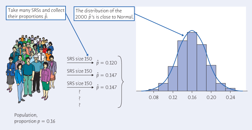
Extensive studies in Ohio have found that the proportion of uninsured drivers is approximately 16%. This is the population proportion.
Figure 15.2 illustrates the process of choosing many samples and finding the sample proportion of uninsured drivers
for each one. Follow the flow of the figure from the population at the left, to choosing an SRS and finding the
for this sample, to collecting together the
’s from many samples. The first sample has
= 0.120. The second sample contains a different 150 people, with
= 0.147, and so on. The histogram at the right of the figure shows the distribution of the values of from 2000 separate SRSs of size 150. This histogram displays the sampling distribution of the statistic
.
 ’s from all the samples, and display the distribution of the
’s. The histogram shows the results of 2000 samples.
’s from all the samples, and display the distribution of the
’s. The histogram shows the results of 2000 samples.339
Sampling Distribution
The sampling distribution of a statistic is the distribution of values taken by the statistic in all possible samples of the same size from the same population.
Strictly speaking, the sampling distribution is the ideal pattern that would emerge if we looked at all possible samples of size 150 from our population. A histogram obtained from a fixed number of trials, like the 2000 trials in Figure 15.2, is only an approximation to the sampling distribution. One of the uses of probability theory in statistics is to obtain sampling distributions without simulation. The interpretation of a sampling distribution is the same, however, whether we obtain it by simulation or by the mathematics of probability.
We can use the tools of data analysis to describe any distribution. Let’s apply those tools to Figure 15.2. What can we say about the shape, center, and spread/variability of this distribution?
-
Shape: It looks Normal! Detailed examination confirms that the distribution of from many samples is very close to Normal.
-
Center: The mean of the 2000
’s is 0.1602. That is, the distribution is centered very close to the population proportion p = 0.16.
-
Spread: The standard deviation of the 2000
’s is 0.0292. The relationship between the standard deviation, the population proportion, and the sample size is described in the next section.
Although these results describe just one simulation of a sampling distribution, they reflect facts that are true whenever we use random sampling.
Apply Your Knowledge
Question 15.6
Generating a Sampling Distribution. Let’s illustrate the idea of a sampling distribution in the case of a very small sample from a very small population. The population is the sex of 10 students in a class:
| Student | 0 | 1 | 2 | 3 | 4 | 5 | 6 | 7 | 8 | 9 |
| Score | F | F | M | M | F | M | M | M | F | M |
The parameter of interest is the proportion of females p in this population. The sample is an SRS of size n = 4 drawn from the population. Because the students are labeled 0 to 9, a single random digit from Table B chooses one student for the sample.
- (a) Find the proportion of females among the 10 students in the population. This is the population proportion p.
- (b) Use technology or the first digits in row 116 of Table B to draw an SRS of size 4 from this population. What is the sex of the four students in your sample? What is the proportion of females
? This statistic is an estimate of p.
- (c) Repeat this process 9 more times, using technology or the first digits in rows 117 to 125 of Table B. Make a histogram of the 10 values of
. You are simulating the sampling distribution of
, with 10 simulations. Is the center of your histogram close to p?
340