15.4 The sampling distribution of !pcapc!
Figure 15.2 suggests that when we choose many SRSs from a population, the sampling distribution of the sample proportions is centered at the population proportion p. The spread/variability depends on both the population proportion p and the sample size n. Here are the facts we need to get started.6
Mean and Standard Deviation of a Sample Proportion
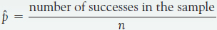
Draw an SRS of size n from a large population that contains proportion p of successes. Let be the sample proportion of successes,
Then:
 The mean of the sampling distribution is p.
-
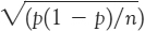
The standard deviation of the sampling distribution is

These results about the mean and the standard deviation of the sampling distribution of  have important implications for statistical inference:
-
The mean of the statistic
is always equal to the mean p of the population. That is, the sampling distribution of is centered at p. In repeated sampling,
will sometimes be above the true value of the parameter p and sometimes below, but there is no systematic tendency to overestimate or underestimate the parameter. This makes the idea of lack of bias in the sense of “no favoritism” more precise. Because the mean of
is equal to p, we say that the statistic
is an unbiased estimator of the parameter p.
unbiased estimator
-
An unbiased estimator is “correct on the average” in many samples. How close the estimator falls to the parameter in most samples is determined by the spread/variability of the sampling distribution. The sample proportion from samples of size n has standard deviation
 . For any population proportion p, the standard deviation of the distribution of gets smaller as we take larger samples. The results of large samples are less variable than the results of small samples.
SAMPLE SIZE MATTERS
The new thing in baseball is using statistics to evaluate players, with new measures of performance to help decide which players are worth the high salaries they demand. This challenges traditional subjective evaluation of young players and the usefulness of traditional measures such as batting average. But success has led many major league teams to hire statisticians. The statisticians say that sample size matters in baseball also: the 162-game regular season is long enough for the better teams to come out on top, but 5-game and 7-game play-off series are so short that luck has a lot to say about who wins.
 The upshot of all this is that we can trust the sample proportion from a large random sample to estimate the population proportion accurately. If the sample size n is large, the standard deviation of
is small, and almost all samples will give values of
that lie very close to the true parameter p. However, the standard deviation of the sampling distribution gets smaller only at the rate
The upshot of all this is that we can trust the sample proportion from a large random sample to estimate the population proportion accurately. If the sample size n is large, the standard deviation of
is small, and almost all samples will give values of
that lie very close to the true parameter p. However, the standard deviation of the sampling distribution gets smaller only at the rate  . To cut the standard deviation of
in half, we must take four times as many observations, not just twice as many. So very precise estimates (estimates with very small standard deviation) may be expensive, time consuming, and impractical.
. To cut the standard deviation of
in half, we must take four times as many observations, not just twice as many. So very precise estimates (estimates with very small standard deviation) may be expensive, time consuming, and impractical.
341
We have described the center and spread of the sampling distribution of a sample proportion
, but not its shape. As the sample size gets larger, the shape of the sampling distribution approaches a Normal distribution for any value of the population proportion.
Sampling Distribution of a Sample Proportion
As the sample size increases, the sampling distribution of becomes approximately Normal. That is, for large n,
has approximately the 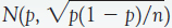 distribution. As a rule of thumb, use this approximation when the sample size n is so large that both np and n(1 − p) are 10 or more.
The accuracy of the Normal approximation improves as the sample size n increases. It is most accurate for any fixed n when p is close to 1/2 and least accurate when p is near 0 or 1. This is why the rule of thumb in the box depends on p as well as n. Here is an example on using the sampling distribution.
EXAMPLE 15.5: The 68–95–99.7 Rule and !pcapc!
Although over 50% of American adults believe the maxim that breakfast is the most important meal of the day, only about 30% eat breakfast daily.7 A cereal manufacturer plans to select an SRS of 1000 American adults. What does the 68–95–99.7 rule tell us about
, the proportion in the sample who eat breakfast every day?

First verify that the rule of thumb to use the Normal approximation is satisfied. Both np = (1000)(0.3) = 300 and n(1 − p) = (1000)(0.7) = 700 are 10 or more. The sampling distribution for
based on an SRS of 1000 is approximately Normal with mean p = 0.3 and standard deviation  . The 68 part of the 68–95–99.7 rule says that 68% of samples of size 1000 should have
within one standard deviation of the mean, or between
. The 68 part of the 68–95–99.7 rule says that 68% of samples of size 1000 should have
within one standard deviation of the mean, or between
(0.3 − 0.014) = 0.286 and (0.3 + 0.014) = 0.314.
Similarly, 95% of samples of size 1000 should have
between
(0.3 − (2)(0.014)) = 0.272 and (0.3 + (2)(0.014)) = 0.328
and almost all samples should have
within 3 standard deviations of the mean, or between 0.258 and 0.342.
In Example 15.2 we estimated the proportion of uninsured drivers in Ohio with an SRS of 150 drivers. How close is this estimate to the true proportion? Here is another example showing how the sampling distribution can be used to begin to answer this question.
EXAMPLE 15.6: How Close Is the Estimate?
STATE: We are conducting a poll to estimate the proportion of Ohio drivers who are uninsured. It is desired to have our sample estimate be within 2% of the population proportion with high probability, say at least 95%. A simple random sample of 150 Ohio drivers will be taken. Is this sample size sufficient to obtain the desired accuracy in our estimate? Or do we need to take a larger sample?

342
PLAN: The true proportion of uninsured drivers in the state is approximately 16%. For our estimate based on an SRS of 150 drivers to be within 2% of the population proportion requires that
be between 14% and 18%. What is the probability that based on an SRS of 150 drivers is between 14% and 18%?
SOLVE: First verify that the rule of thumb to use the Normal approximation is satisfied. Both np = (150)(0.16) = 24 and n(1 − p) = (150)(0.84) = 126 are 10 or more. The sampling distribution for a proportion says that the sample proportion
of uninsured drivers based on a sample of 150 from a population in which 16% of all drivers are uninsured has approximately the Normal distribution with mean equal to the population mean p = 0.16 and standard deviation
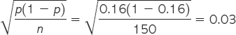
The distribution of
is therefore approximately N(0.16, 0.03).
Using this Normal distribution, the probability we want is

Software gives this probability immediately, or you can standardize and use Table A. For example,
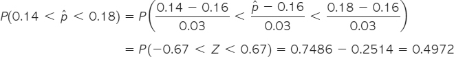
with the usual roundoff error.
CONCLUDE: If you sample 150 drivers, the probability that your sample proportion is within 2% of the population proportion is only about 50%. To increase this probability to at least 95%, it is necessary to take a larger sample.
Example 15.6 raises two important issues. The first is “How do we determine the necessary sample size so that our estimate is within a certain percentage of the true value with a high probability?” The second issue is more subtle. In Example 15.6, the value of the population proportion p was used in our calculation of the accuracy of the estimate. In practice, the value of p is unknown or there would be no need to estimate it. These issues will be addressed in the next chapter, which presents confidence intervals for a population proportion, our first methodology for statistical inference.
Apply Your Knowledge
Question 15.7
Lead-Based Paint. The U.S. Environmental Protection Agency defines lead-based paint as any paint that contains more than 0.5% lead by weight (or about 1 milligram per square centimeter of painted surface). This is the “Action Level” at which the EPA recommends removal of lead paint if it is deteriorating and chipping. A government survey plans to estimate the proportion of schools in your state that exceed the Action Level. The researchers will report the proportion
from their sample as an estimate of the population proportion p.
- (a) Explain to someone who knows no statistics what it means to say that
is an “unbiased” estimator of p.
- (b) The sample result
is an unbiased estimator of the population proportion p no matter what size SRS the study uses. Explain to someone who knows no statistics why a large sample gives more trustworthy results than a small sample.
343
Question 15.8
Larger Sample, More Accurate Estimate. About 90% of young adult Internet users (ages 18 to 29) use social-networking sites.8
- (a) Suppose a sample survey contacts an SRS of 1500 young adult Internet users and calculates the proportion
in this sample who use social-networking sites. What is the approximate distribution of
? What is the probability that
is between 87% and 93%? This is the probability that
estimates p within 3%.
- (b) If the sample size were 6000 rather than 1500, what would be the approximate distribution of
? Now what is the probability that
falls within 3% of p? The larger sample size is much more likely to give an accurate estimate of p.
Question 15.9
Teen Binge Drinking. In 2012, about 24% of high school seniors reported binge drinking (defined as 5 or more drinks in a row in the past 2 weeks), a substantial drop since the late 1990s.9 An SRS of 500 high school seniors is to be taken.
- (a) What is the standard deviation of
, the proportion of high school seniors in the sample who would report binge drinking?
- (b) How large a sample is required to reduce the standard deviation of
to 0.01?