Chapter 1. One- and Two-dimensional Motion
Objective

The objectives of the first part this experiment are to investigate the one-dimensional motion of a body released from rest in free fall, and to measure the acceleration of the body due to gravity. In the second part of this experiment you will investigate the projectile motion of an object launched with an initial velocity in a vertical plane and to determine the independence of the motion of the body along two perpendicular axes.
Theory
2.1 Motion with Constant Acceleration
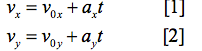
If the motion is constrained in two dimensions, then the velocity components in the x- and y- directions can be expressed as:
These two equations can be combined into a single vector equation (symbols in bold type are vectors):

Where v = vxi + vyj and a = axi + ayj. The position of the particle in the x- and y-directions can be expressed as:

Equations [4] and [5] can be combined into a single vector equation:
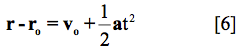
In the above equations ro = xoi + yoj and vo= voxi + voyj are, respectively, the initial (t = 0.0 sec) position and the initial velocity of the particle with r and v being the corresponding position and velocity at time t. Also notice in the above equations that the position and velocity components in a given direction are affected by the acceleration in that direction alone. Thus the motions in the x- and y-directions are independent of each other.
2.2 One-Dimensional Motion (Free Fall)
A particle is said to be under free fall when the only force acting on it is due to gravity. The free-fall motion of a particle is described by eqs. [2] and [5]
2.3 Two-Dimensional Motion (Projectile Motion)
If an object is launched at an angle θ above the horizontal, the resulting two-dimensional motion is equivalent to superimposition of two one-dimensional motions. The two one- dimensional motions can be described by the following equations where g is the acceleration due to gravity and assumed constant.

2.4 A Word about Numerical Differentiation
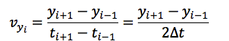
Theoretically, the instantaneous speed v(t) of a particle moving along the y-axis is defined as:
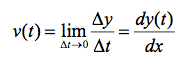
In practice, the time interval Δt has to be finite. There is an instrument-related limit to how small the time interval can be. Thus, experimentally the instantaneous speed is calculated by numerical differentiation. This amounts to calculating the average speed between two points using as small a time interval as possible.
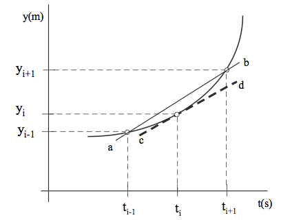
Consider the plot of position vs. time (the parabolic curve) for an object in Figure 1. The slope of the line ab equals:
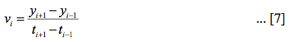
This slope of line ab is the average speed of the object in the time interval Δt = t i+1 – t i-1. As the time interval Δt is reduced to nearly zero, the slope of ab will approach the slope of the tangent cd. The slope of cd is the instantaneous speed of the object at the instant ti. We will use the approximation that the value of the average speed in the interval Δt = t i+1 – t i-1 can be considered as the speed of the particle at ti.
Experimental
3.1 An Overview
To study the one-dimensional motion you will take a video (record the motion using a digital camera) of a ball dropped from about 1.5 to 2.0 m. The recording and analysis of the video involves two pieces of software: [1] VideoPoint Capture software for controlling the video camera and capturing the video and [2] VideoPoint Physics Fundamentals software to analyze the data. The recorded video is a series of digital images (video frames) with a known time interval between two consecutive frames. The analysis software generates a list of x- and y-coordinates as a function of time. This position vs. time data is exported to a spreadsheet to compute velocity and acceleration as a function of time for the particle. This procedure is then repeated for a particle in projectile motion.
To study the two-dimensional motion a video will be recorded for a ball launched at an angle θ above the horizontal.
In our analyses we will neglect the air resistance. For a constant acceleration due to gravity, a plot of y-position vs. time would be a parabola. You can determine the acceleration due to gravity by fitting a second order polynomial to this parabola (eq.5).A plot of y-component of velocity versus time should yield a straight line (eq.2) the slope of which is the acceleration due to gravity.
1.0.1 Experimental Details
3.2.1 Capturing the Video Clip
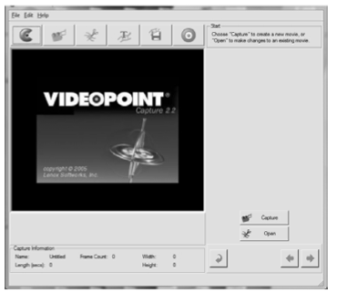
- Click on the VideoPoint Capture icon (see Fig.2) on the computer screen, the opening screen is shown in Fig.3 below.
- Turn on the camera and from the Scene Selection Menu select SPORTS (this corresponds to a shutter speed of 1/250 sec.).
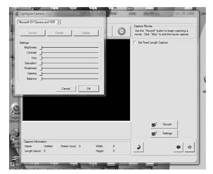
- Click on the Capture Button. This should bring up a screen as shown in Figure 4. You should see the video input from the camera. If you do not see any video input but instead see a black screen, do the following:[a] click on the settings button which brings a pop-up window with a drop down menu with a list of cameras attached to the computer along with other camera settings;[b] Choose the proper camera and press the OK button. If the screen still looks black, make sure the camera is on, then press record, then press stop, and finally press the back arrow.
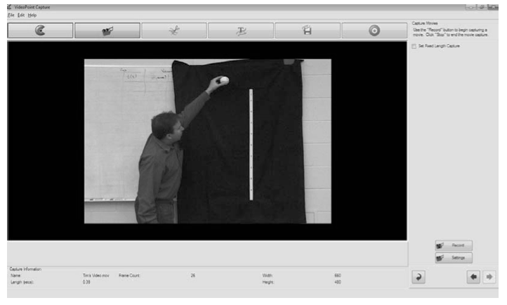
- You are now ready to collect the data by capturing a video. One team member can either hold a meter stick or you can mount it on the wall using sticky tape. Get the digital video camera ready for recording by hitting the Record button. During recording, the Settings button will be “grayed out” and the Record Button will become a Stop button (This is a dual function control button and switches back and forth between Record and Stop). Now, drop a ball from a height of about 1.5 to 2.0 meters. Press the Stop button after the ball hits the ground. This is it – you have collected all the data you need for studying the one-dimensional motion. The recorded video may now be edited with the VideoPoint Capture Software.
- After pressing the Stop button, save the video clip as a .mov movie file using the File drop down menu at the top of the screen.
Experimental Details (cont'd)
3.2.2 Editing the Video Clip
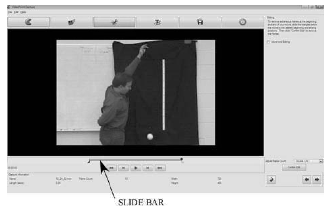
- There will be many empty frames in the video you just recorded. Before you begin data analysis, the video will be cropped to include only the frames of interest. After the STOP button is pressed, the editing screen will appear. The editing screen will show a set of controls similar to the controls you see on a typical DVD player. When the play button is pressed, the video will begin to play, and the button is transformed into a stop button. These controls are shown in Figure 7. There is a slide bar with a black diamond on the top. You can advance/recede the video clip by sliding the black diamond along the slide bar. Using these controls you can review the film clip to decide where to crop the video clip. The two white triangles on the slide bar are used to mark the start and the end of the frames that are to be analyzed.
- Review the video clip and then use the white triangles to mark the start and finish of the frames that you want to analyze. Mark the start of the clip after the ball has been released and cleared the hand of the person dropping the ball. This may require deleting 4 - 6 frames after the ball is released. Once you have chosen the start and finish points on the clip, click on the Confirm Edit button. This will crop the video clip to give you the desired frames of interest for further analysis. You can now save the cropped clip.
1.1 Experimental Details (cont'd)
3.3 Analyzing the Video Clip:
- Open the VideoPoint Physics Fundamentals Software, and using the File drop down menu, load the video clip movie file saved in the last step.
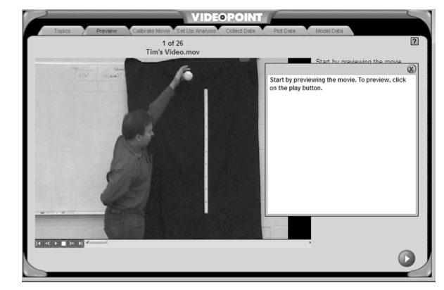
- The first screen - labeled as the Preview Screen in the tabs at the top of the screen - is used to view the video clip. The tabs are used to navigate through the program. As each screen progresses a hint will appear in a pop-up window. These hints can be closed using the X button in the upper, right hand corner of the pop-up window. Once the clip has been viewed, advance to the next screen using the forward arrow button.
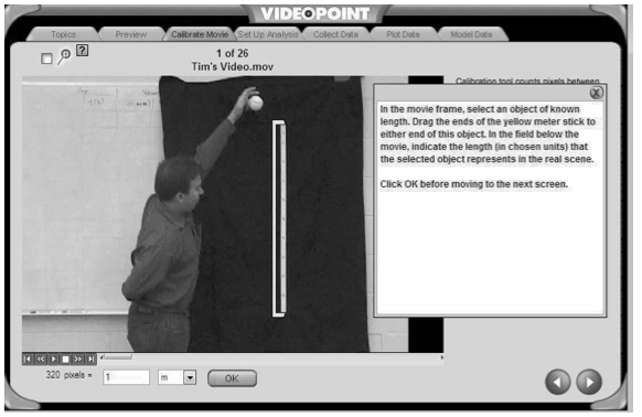
- This screen is the calibrate screen (Figure 9) and is used to provide a length scale to the system. Move one end of the yellow calibration tool to align with one end of the meter stick and move the other end of the calibration tool to align with the other end of the meter stick. Enter the length of the object between the jaws of the calibration tool (1.0 meter if you used 0.0 and 100.0 cm marks on the meter stick). Advance to the next screen.
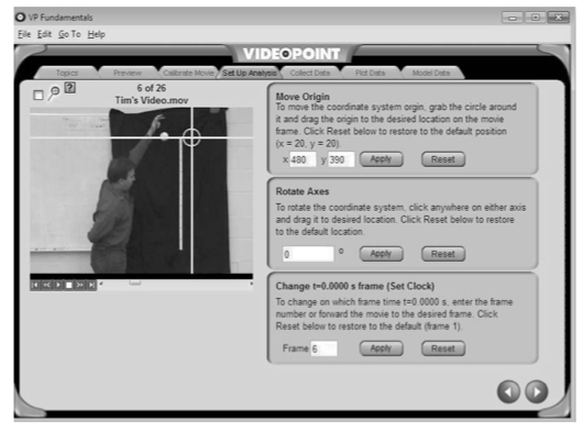
- The Set-Up Analysis frame. Set the origin using Move Origin x- and y-position boxes. The axis may also be rotated and the t = 0.0 sec frame may also be set. Go to the next frame.
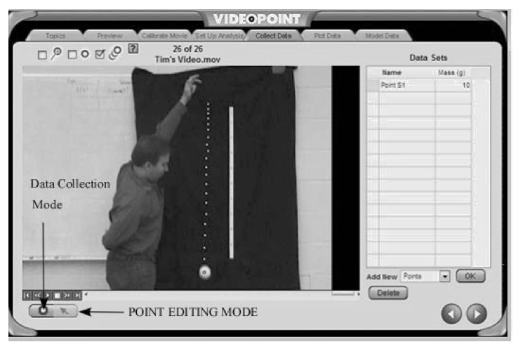
- The Collect Data screen. You can use the mouse to select data points on the screen while in the Data Collection Mode. As the data point is selected, the video clip advances to the next frame. The set of data points may be completely deleted by selecting the data set name (e.g., Points S1) and pressing the Delete button. A new set may be started with the Add New Points drop down menu and hitting the OK button. Point locations may be moved while in the Point Editing Mode. When in the Point Editing Mode, the mouse can grab the point and drag it to a new position. Once all the points have been selected, you can move to the next screen. You should now export the data into a spreadsheet file using the File menu at the top of the screen.
1.2 Experimental Details (cont'd)
3.4 Analyzing the Data Collected (Free Fall)
- Open the spreadsheet containing the data.
- Plot the y-position vs. time data. Add a trend line using a second order polynomial fit. Show the equation of the line and the R-squared valued.
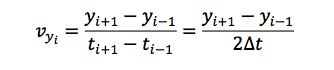
- Compute the y-component of the velocity using the equation:
- Plot the y-component of the velocity vs. time. Add a trend line with a linear fit. Show the equation of the line and the R-squared value.
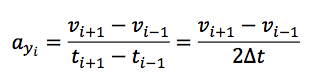
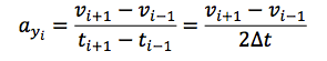
- Compute the y-component of the acceleration using the equation:
- Plot the y-component of the acceleration versus time. Add a trend line with a linear fit. Show the equation of the line and the R-squared value.
1.3 Experimental Details (cont'd)
3.5 Analyzing the Data Collected (Projectile Motion)
- Have one of the lab partners toss the ball at an angle and with an initial velocity. To record and analyze the video follow the procedure you used for the one-dimensional motion.
- Open the spreadsheet containing the data collected.
- Plot the y-position versus time data. Add a trend line using a second order polynomial fit. Show the equation of the line and the R-squared valued.
- Calculate the y-component of the velocity using the equation:
- Plot the y-component of the velocity vs. time. Add a trend line with a linear fit. Show the equation of the line and the R-squared value.
- Calculate the y-component of the acceleration using the equation:
- Plot the y-component of the acceleration versus time. Add a trend line with a linear fit. Show the equation of the line and the R-squared value.
- Plot the x-position versus time data. Add a trend line using a linear fit. Show the equation of the line and the R-squared valued.
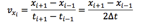
- Calculate the x-component of the velocity using the equation:
- Plot the x-component of the velocity versus time. Add a trend line with a linear fit. Show the equation of the line and the R-squared value.
Pre-Lab Assessment
1. A particle is launched in a gravitational field g with an initial velocity vo at an angle of θ with respect to the horizontal.
Question a.
XlqVDDankx/9T3U1fOgjocOsbqohRknb5m+4reWrNiQlsktM9Awtmabopm2oWm1ftw/H1nzmnGlOUT0TrMfBxbqfLVXpx59M3AZD+CH9NYbmrrKysg9JnVLlNnWKzuKiEawfomBvTbskM/7gvpQpYbeCop39luvGgIGFbyzXL3G+eZEfee+H2NGz9kD5hp1WuHhk6A==Question b.
oa4QntOu6REKKU8UE7Vj2X7eDrkBqdQc3P2oJUU4ZvNt4tXgyka56pB3KnJr8hxmY1KeQGGDE2uptOGOgrlPoEskAXvQo93cDQuSTeAwfFrkKgayyZiOzNxoVmZn3pzrbgrTleaH5fQtKNf5YsrTxZadggiee9+0DzNevvUYculjfgps3m7+RO/K9c0OMkCIcoubOoOTXJuilQgOiQqqevO5IuKDbstZKf4Cb4r4ZJLjtjMf3L81BNfOULo3/ad1gKCB0WUY9MHR6vPlr0y5rQGLdGkuRiQVTxy76A==In the table below are listed values of y(t) =Ct2 where C is a constant. Fill out the last column (use an Excel spreadsheet) using eq.[7]. Plot y(t) vs. t and fit a second order polynomial to the data points. From the fitting parameters, determine the value of C. Plot v(t) vs. t add a trend line with a linear fit to determine the acceleration of the particle. How is C related to the acceleration of the particle?
Question
| t in sec | y(t) in m | v(t) in m/s | |
|---|---|---|---|
| 1 | 0 | 0 | IUdMjE7Xrqo= |
| 2 | 0.1 | 0.05 | IUdMjE7Xrqo= |
| 3 | 0.2 | 0.2 | IUdMjE7Xrqo= |
| 4 | 0.3 | 0.45 | IUdMjE7Xrqo= |
| 5 | 0.4 | 0.8 | IUdMjE7Xrqo= |
| 6 | 0.5 | 1.25 | IUdMjE7Xrqo= |
| 7 | 0.6 | 1.8 | IUdMjE7Xrqo= |
| 8 | 0.7 | 2.45 | IUdMjE7Xrqo= |
| 9 | 0.8 | 3.2 | IUdMjE7Xrqo= |
| 10 | 0.9 | 4.05 | IUdMjE7Xrqo= |
| 11 | 1 | 5 | IUdMjE7Xrqo= |
| 12 | 1.1 | 6.05 | IUdMjE7Xrqo= |
| 13 | 1.2 | 7.2 | IUdMjE7Xrqo= |
| 14 | 1.3 | 8.45 | IUdMjE7Xrqo= |
| 15 | 1.4 | 9.8 | IUdMjE7Xrqo= |
| 16 | 1.5 | 11.25 | IUdMjE7Xrqo= |
Data Report
Click here to download Data Report Printable PDF
JUST FOR THE FUN OF IT
Click here to open Just for the Fun of It PDF.