15.1 Vector Fields
974
OBJECTIVES
When you finish this section, you should be able to:
- Describe a vector field (p. 974)
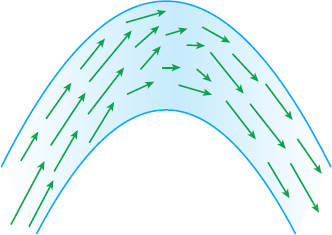
Suppose you are studying the motion of a fluid such as water or air. The fluid is composed of a multitude of moving particles. At any instant of time \(t\), each particle is at a given point and is moving with a particular velocity \(\mathbf{v}(t) .\) If we assign a velocity vector to each particle at time \(t\) and take a picture at that instant, then the snapshot of all the vectors at this time \(t\) forms a vector field. Figure 1 shows a possible vector field for the velocity of water in a river as it flows around a bend.
In Chapter 11, we discussed vector functions, \(\mathbf{r}=\mathbf{r}(t)\), \(a\leq t\leq b\). A vector function associates a vector \(\mathbf{r}\) to a real number \(t\). A vector field is a function that associates a vector to a point in the plane or to a point in space. That is, a vector field is a function whose domain is a set of points in the plane or in space and whose range is a set of vectors.
spanDEFINITIONspan Vector Field
Let \(P=P(x,y)\) and \(Q=Q(x,y)\) be functions of two variables defined on a subset \(R\) of the \(xy\)-plane. A vector field \(\mathbf{F}\) over \(\boldsymbol R\) is defined as the function \[ {\bbox[5px, border:1px solid black, #F9F7ED]{\bbox[#FAF8ED,5pt]{ \mathbf{F}=\mathbf{F}(x,y)=P(x,y)\mathbf{i}+Q(x,y) \mathbf{j} }}} \]
Let \(P=P(x,y,z)\), \(Q=Q(x,y,z)\), and \(R=R(x,y,z)\) be functions of three variables defined on a subset \(E\) of space. A vector field \(\mathbf{F}\) over \(\boldsymbol E\) is defined as the function \[ {\bbox[5px, border:1px solid black, #F9F7ED]{\bbox[#FAF8ED,5pt]{ \mathbf{F}=\mathbf{F}(x,y,z)=P(x,y,z)\mathbf{i} +Q(x,y,z)\mathbf{j}+R(x,y,z)\mathbf{k} }}} \]
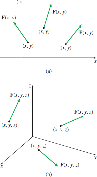
The vector field \(\mathbf{F}=\mathbf{F}(x,y)\) consists of vectors in the plane with initial points at \((x,y)\). In general, it is not possible to draw a vector for each point \((x,y) \) in the domain, so a representative set of vectors (arrows) are drawn. See Figure 2(a).
Similarly, the vector field \(\mathbf{F}=\mathbf{F}(x,y,z)\) consists of vectors in space with initial points at \((x,y,z)\). See Figure 2(b).
1 Describe a Vector Field
Describing a Vector Field in the Plane
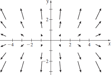
Describe the vector field \(\mathbf{F}=\mathbf{F}(x,y)=-y\mathbf{i}+x\mathbf{j}\) by drawing some of the vectors \(\bf{F}.\)
Solution We begin by making a table of vectors. We do this by choosing points \((x,y) \) and finding the values of \(\bf{F.}\)
| \((x,y)\) | \(( 2,0)\) | \(( 0,2)\) | \(( -2,0)\) | \(( 0,-2)\) | \(( 3,3)\) | \(( -3,3)\) | \(( -3,-3)\) | \(( 3,-3)\) |
|---|---|---|---|---|---|---|---|---|
| \(\mathbf{F}(x,y) \) | \(\ 2\mathbf{j}\) | \(-2\mathbf{i}\) | \(-2\mathbf{j}\) | \(2\mathbf{i}\) | \(-3\mathbf{i}+3\mathbf{j}\) | \(-3\mathbf{i}-3\mathbf{j}\) | \(3\mathbf{i}-3\mathbf{j}\) | \(3\mathbf{i}+3\mathbf{j}\) |
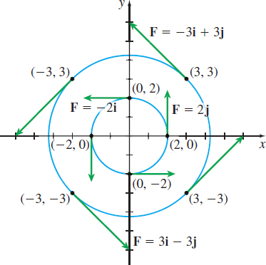
Figure 3 illustrates the vectors from the table. Notice that each vector in the field is tangent to a circle centered at the origin, and the direction of the vectors indicates that the field is rotating counterclockwise. This field might represent the motion of a wheel spinning on an axle, with each vector equal to the velocity at a point of the wheel.
NOW WORK
Problem 7.
975
Describing a Vector Field in Space
Describe the vector field \(\mathbf{F}=\mathbf{F}(x,y,z)=y\bf{j}\) by drawing some of the vectors \(\bf{F}.\)
Solution Several vectors from the vector field are listed in the table below.
| \(( x,y,z)\) | \(( 0,0,0) \) | \(( 0,1,1)\) | \(( 0,1,2)\) | \(( 0,-1,-1)\) | \((1,-1,0) \) | \(( 1,3,1) \) | \(( 1,-2,-1))\) |
|---|---|---|---|---|---|---|---|
| \(\bf{F}( x,y,z) \) | \(\bf{0}\) | \(\bf{j}\) | \(\bf{j}\) | \(-\bf{j}\) | \(-\bf{j}\) | \(3\bf{j}\) | \(-2\bf{j}\) |
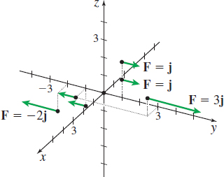
Each vector in the vector field \(\bf{F}\) is parallel to the \(y\)-axis. The magnitude of the vector equals \(\left\vert y\right\vert \) and is proportional to the distance of the vector from the \(xz\)-plane. See Figure 4.
NOW WORK
Problem 13.
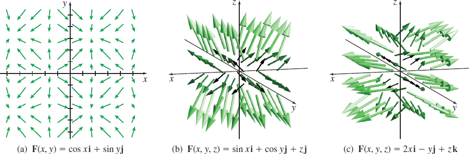
The vector fields in Examples 1 and 2 were relatively easy to graph by hand. But this is not true for most vector fields, particularly for vector fields in space. There is graphing technology, often found in computer algebra systems, however, with the capability of drawing vector fields. If you have technology available, use it to visualize the vector fields in the text, and to experiment with graphing vector fields. See Figure 5 for some examples.
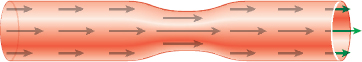
Describing a Vector Field–Blood Flow
An example of a velocity field arises in describing the flow of a fluid through a pipe or the flow of blood through an artery. At each point inside the pipe (or the artery), a vector is defined that represents the velocity of the flow. See Figure 6. The magnitude of each vector represents the speed of the fluid’s flow. Notice that the speed of blood flow is slower near the artery wall and is faster near the center of the artery and that the speed increases where the artery is contracted.
Describing a Vector Field–Newton’s Law of Gravitation
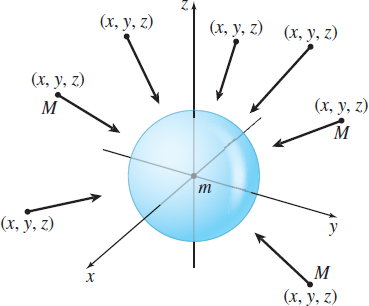
A gravitational field is defined by the vector field \[ {\bbox[5px, border:1px solid black, #F9F7ED]{\bbox[#FAF8ED,5pt]{{ \mathbf{F}=\mathbf{F}(x,y,z)=-\dfrac{{\boldsymbol G}m{\boldsymbol M}}{x^{2}+y^{2}+z^{2}}\mathbf{u} }}}} \]
where \(m\) and \(M\) are the masses of two objects, one located at the origin \((0,0,0)\) and the other at the point \((x,y,z)\); \(G\) is the gravitational constant; and \(\mathbf{u}\) is a unit vector in the direction from \((0,0,0)\) to \((x,y,z)\). Here, \(\mathbf{F}\) is the force of attraction between the two objects. The force vectors \(\mathbf{F}\) are directed from the object at \((x,y,z)\) toward the object at \((0,0,0)\). Figure 7 illustrates a gravitational field.
976
Describing a Vector Field–Coulomb’s Law
An electric force field is defined by the vector field \[ {\bbox[5px, border:1px solid black, #F9F7ED]{\bbox[#FAF8ED,5pt]{{ \mathbf{F}=\mathbf{F}(x,y,z)=\dfrac{\varepsilon qQ}{x^{2}+y^{2}+z^{2}}\mathbf{u} }}}} \]
where \(\varepsilon \) is a positive constant that depends on the units being used; \(q\) and \(Q\) are the charges of two objects, one located at the origin \((0,0,0)\) and the other at the point \((x,y,z)\); and \(\mathbf{u}\) is the unit vector in the direction from \((0,0,0)\) to \((x,y,z)\). Here, \(\mathbf{F}\) is the electric force exerted by the charge at \((0,0,0)\) on the charge at \((x,y,z)\). For like charges, we have \(qQ>0\) and the force \(\mathbf{F}\) is repulsive. For unlike charges, we have \(qQ<0\) and the force \(\mathbf{F}\) is attractive.
Recall that the gradient \(\boldsymbol\nabla\! f\) of a function \(f=f(x,y) \) in the plane is the vector \[ {\bbox[5px, border:1px solid black, #F9F7ED]{\bbox[#FAF8ED,5pt]{{ \boldsymbol\nabla\! f(x,y)=f_{x}(x,y)\mathbf{i}+f_{y}(x,y)\mathbf{j} }}}} \]
and the gradient \(\boldsymbol\nabla\! f\) of a function \(w=f( x,y,z) \) in space is the vector \[ {\bbox[5px, border:1px solid black, #F9F7ED]{\bbox[#FAF8ED,5pt]{{ \boldsymbol\nabla\! f(x,y,z)=f_{x}(x,y,z)\mathbf{i}+f_{y}(x,y,z) \mathbf{j}+f_{z}(x,y,z)\mathbf{k} }}}} \]
We see that the gradient \(\boldsymbol\nabla\! f\) of a function \(f\) is a vector field, called the gradient vector field.
Describing a Gradient Vector Field
- Find the gradient vector field of \(f(x,y)=x^{2}+4y^{2}\) and graph it by drawing some of the vectors \(\boldsymbol\nabla\! f\).
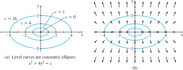
- Graph the level curves \(f(x,y)=c\), for \(c=0,1,4\), and 16.
Solution (a) The gradient of \(f\) is \(\boldsymbol\nabla\! f=\dfrac{\partial f}{\partial x}\,\mathbf{i}+\dfrac{\partial f}{\partial y}\,\mathbf{j}=2x\mathbf{i}+8y\mathbf{j}\). The graph of the gradient vector field is shown in Figure 8.
(b) Figure 9(a) illustrates the level curves of the elliptic paraboloid \(f(x, y)=x^{2}+4y^{2}=c\) for \(c=0,1,4\), and 16. Compare the level curves with the gradient vector field illustrated in Figure 8. Notice that the gradient vectors are orthogonal to the level curves, as shown in Figure 9(b).