16.2 Separation of Variables in First-Order Differential Equations
1062
OBJECTIVES
When you finish this section, you should be able to:
- Solve a separable first-order differential equation (p. 1062)
- Identify a homogeneous function of degree \(k\) (p. 1063)
- Use a change of variables to solve a homogeneous first-order differential equation (p. 1064)
- Solve applied problems (p. 1066)
In this section, we solve first-order differential equations that are separable. Such differential equations are used to find orthogonal trajectories of families of curves and to analyze inhibited growth models, such as bacterial growth and sales forecasts of a company.
A first-order differential equation is usually written in the form \[\bbox[5px, border:1px solid black, #F9F7ED]{\bbox[#FAF8ED,5pt] {\dfrac{dy}{dx}=f(x,y)} } \]
where \(f\) is continuous on its domain. If we treat \(dy\) and \(dx\) as differentials, we can write \(\dfrac{dy}{dx}=f( x,y) \) in differential form as \[\bbox[5px, border:1px solid black, #F9F7ED]{\bbox[#FAF8ED,5pt] {M(x,y)\,dx+N(x,y)\,dy=0} } \]
where \(M\) and \(N\) are each continuous on their domains.
spanDEFINITIONspan Separable Equation
A first-order differential equation is said to be separable if it can be written in the form \[\bbox[5px, border:1px solid black, #F9F7ED]{\bbox[#FAF8ED,5pt] {M(x)\,dx+N(y)\,dy=0} } \]
where \(M\) is a function of \(x\) alone, \(N\) is a function of \(y\) alone, and both \(M\) and \(N\) are continuous on their domains.
1 Solve a Separable First-Order Differential Equation
The following steps are used to solve separable differential equations:
Steps for Solving a Separable Differential Equation
Step 1 Express the given equation in the differential form \[ \begin{equation*} M(x)\,dx+N(y)\,dy=0 \end{equation*} \]
Step 2 Integrate to obtain the general solution \[ \begin{equation*} \int M(x)\,dx+\int N(y)\,dy=C \end{equation*} \]
where \(C\) is the constant of integration.
1063
Solving a Separable First-Order Differential Equation
Solve \(\dfrac{dy}{dx}=\dfrac{2e^{x}}{y^{2}}\)
Solution Use the steps from above:
Step 1 Express \(\dfrac{dy}{dx}=\dfrac{2e^{x}}{y^{2}}\) in the differential form: \[ y^{2}dy-2e^{x}dx=0\qquad \hbox{or equivalently, as}\qquad y^{2}dy=2e^{x}dx \]
Step 2 Integrate to obtain the general solution. \[ \begin{eqnarray*} \int y^{2}dy &=&\int 2e^{x}dx \\ \dfrac{y^{3}}{3} &=&2e^{x}+C \end{eqnarray*} \]
where \(C\) is a constant. This solution is expressed implicitly. To obtain the explicit form, solve for \(y.\) \[ \begin{eqnarray*} y^{3} &=&6e^{x}+3C \\ y &=&\sqrt[3]{6e^{x}+3C} \end{eqnarray*} \]
NOW WORK
Problems 5 and 15.
2 Identify a Homogeneous Function of Degree \(k\)
Some first-order differential equations are not separable, but can be made sparable by a change of variable. This is true for differential equations of the form \(\dfrac{dy}{dx}=f(x,y)\), where \(f\) is a homogeneous function.
spanDEFINITIONspan Homogeneous Function of Degree \(k\)
A function \(f(x,y)\) is said to be a homogeneous function of degree \(k\) in \(x\) and \(y\) if, and only if, for \(t>0\), \[\bbox[5px, border:1px solid black, #F9F7ED]{\bbox[#FAF8ED,5pt] {f(tx,ty)=t^{k}f(x,y)} } \]
for some real number \(k\).
Identifying a Homogeneous Function of Degree \(k\)
- \(f(x,y)=3x^{2}-xy+y^{2}\) is a homogeneous function of degree 2, since \[ \begin{eqnarray*} f(tx,ty)& =&3(tx)^{2}-( tx) ( ty) +(ty)^{2}=t^{2}3x^{2}-t^{2}xy+t^{2}y^{2} \\ & =&t^{2}(3x^{2}-xy+y^{2})=t^{2}f(x,y)\quad \hbox{for all }t>0 \end{eqnarray*} \]
- \(f(x,y)=\sqrt{x+4y}\) is a homogeneous function of degree \(\dfrac{1}{2}\), since \[ \begin{eqnarray*} f(tx,ty)&=&\sqrt{tx+4( ty) }=\sqrt{t(x+4y)}=\sqrt{t}\sqrt{x+4y}\\ &=&t^{1/2}f(x,y)\quad \hbox{for all }t>0 \end{eqnarray*} \]
- \(f(x,y)=\dfrac{x}{\sqrt{x^{2}-y^{2}}}\) is a homogeneous function of degree \(0\), since \[ \begin{eqnarray*} f(tx,ty)&=&\frac{tx}{\sqrt{(tx)^{2}-(ty)^{2}}}=\frac{tx}{\sqrt{t^{2}(x^{2}-y^{2})}}=\frac{tx}{t\sqrt{x^{2}-y^{2}}}\\ &=&t^{0}f(x,y)\quad \hbox{for all }t>0 \end{eqnarray*} \]
- \(f(x,y)=x-y^{2}\) is not a homogeneous function, since \[ f(tx,ty)=tx-(ty)^{2}=t(x-ty^{2})\neq t^{k}(x-y^{2}) \] for all \(t>0\) and some \(k\)
NOW WORK
Problem 21.
1064
spanDEFINITIONspan Homogeneous First-Order Differential Equation
A first-order differential equation of the form \[\bbox[5px, border:1px solid black, #F9F7ED]{\bbox[#FAF8ED,5pt] {M(x,y)\,dx+N(x,y)\,dy=0} }\]
is said to be homogeneous if \(M\) and \(N\) are homogeneous functions of the same degree.
NOTE
The word “homogeneous” has been used in two different ways: to describe a property of a function and to identify a certain type of first-order differential equation. Context will make it clear which meaning applies.
3 Use a Change of Variables to Solve a Homogeneous First-Order Differential Equation
To solve first-order homogeneous differential equations, we use the following change of variables theorem.
THEOREM Change of Variables for Homogeneous First-Order Differential Equations
If \(M(x,y)\,dx+N(x,y)\,dy=0\) is a homogeneous first-order differential equation, then it can be transformed into a first-order differential equation whose variables are separable by using the substitution \[\bbox[5px, border:1px solid black, #F9F7ED]{\bbox[#FAF8ED,5pt] {y=xv( x)} } \]
where \(v=v( x) \) is a differentiable function of \(x\).
NOTE
For simplicity of notation, we usually write \(v\) instead of \(v( x)\).
Proof
In the differential equation \(M( x,y)\,dx+N( x,y)\,dy=0,\) we use the substitution \(y=xv,\) where \(v=v( x) \) is a differentiable function of \(x\). Then \(dy=x\,dv+v\,dx\) and \[ \begin{equation*} M(x,y)\,dx+N(x,y)\,dy=M(x,xv)\,dx+N(x,xv)(x\,dv+v\,dx)=0 \end{equation*} \]
Since \(M\) and \(N\) are each homogeneous functions of degree \(k\), it follows that for some number \(k\) \[ \begin{eqnarray*} x^{k}M(1,v)\,dx+x^{k}N(1,v)(x\,dv+v\,dx)& =&0\qquad \color{#0066A7}{{M ( x,}\, {xv} {) =x^{k}M (1,}\, {v} {){,}}}\\ &&\phantom{0}\qquad \color{#0066A7}{{N (x,}\, {xv} {) =x^{k}N(1,}\, {v} {)}} \\ x^{k}\left[ M( 1,v)\,dx+N( 1,v) ( x\,dv+v\,dx) \right] & =&0 \\ M(1,v)\,dx+N(1,v)x\,dv+N(1,v)v\,dx& =& 0\qquad \color{#0066A7}{{\hbox{Divide out } x^{k}.}} \\ \lbrack M(1,v)+vN(1,v)]\,dx+N(1,v)x\,dv& =&0 \\ \frac{dx}{x}+\frac{N(1,v)}{M(1,v)+vN(1,v)}dv& =&0 \end{eqnarray*} \]
provided neither denominator is \(0\). This first-order differential equation is separable.
Steps for Solving a Homogeneous First-Order Differential Equation \({M(x,y)\,dx\,+\, N(x,y)\,dy=0}\)
Step 1 Confirm that the functions \(M\) and \(N\) are homogeneous of the same degree.
Step 2 Let \(y=xv\). Substitute for \(y\) and \(dy=x\,dv+v\,dx.\)
Step 3 Express the new equation in differential form. The variables will be separable.
Step 4 Integrate to obtain the general solution and replace \(v\) by \(\dfrac{y}{x}.\)
1065
Solving a Homogeneous First-Order Differential Equation
Solve the differential equation \((x^{2}-3y^{2})\,dx+2xy\,dy=0\).
Solution Follow the steps for solving a homogeneous first-order differential equation.
Step 1 Both \(x^{2}-3y^{2}\) and \(2xy\) are homogeneous of degree 2. Do you see why?
Step 2 Let \(y=xv\). Then \(dy=x\,dv+v\,dx\). Substitute these into the differential equation: \[ \begin{eqnarray*} (x^{2}-3y^{2})\,dx+2xy\,dy& =&0 \\ [ x^{2}-3( xv) ^{2}]\,dx+2x (xv) (x\,dv+v\,dx)& =&0\qquad \color{#0066A7}{{dy=x\,} {dv=} {+} {v} {dx}} \\ ( x^{2}-x^{2}v^{2})\,dx+2x^{3}v\,dv& =&0 \\ x^{2}(1-v^{2})\,dx+2x^{3}v\,dv& =&0 \end{eqnarray*} \]
Step 3 Then for \(x\neq 0\) and \(v\neq \pm 1,\) we can separate the variables by dividing by \(x^{3}\) and \(1-v^{2}\). \[ \begin{eqnarray*} x^{2} ( 1-v^{2})\,dx+2x^{3}v\,dv &=&0 \\ \hspace{-2pc}\dfrac{x^{2}( 1-v^{2})\,dx}{x^{3}( 1-v^{2}) }+\dfrac{2x^{3}v\,dv}{x^{3}( 1-v^{2}) } &=&0 \\ \dfrac{dx}{x}+\dfrac{2v\,dv}{1-v^{2}} &=&0 \end{eqnarray*} \]
Step 4 Integrate. \[ \begin{eqnarray*} \hspace{-5pc}\int \frac{dx}{x}-\int \frac{2v\,dv}{v^{2}-1} &=&0\\ \ln \left\vert x\right\vert -\ln \left\vert v^{2}-1\right\vert &=&C_{1} \\ \ln \left\vert \dfrac{x}{v^{2}-1}\right\vert &=&C_{1} \end{eqnarray*} \]
Since \(C_{1}\) is a constant, we can write \(C_{1}=\ln C_{2},\) where \(C_{2}\) is a constant. Then \[ \begin{eqnarray*} \ln \left\vert \dfrac{x}{v^{2}-1}\right\vert &=&\ln C_{2} \\ \left\vert \dfrac{x}{v^{2}-1}\right\vert &=&C_{2} \\ \left\vert \dfrac{x}{\dfrac{y^{2}}{x^{2}}-1}\right\vert &=&C_{2}\qquad \color{#0066A7}{{v}} \color{#0066A7}{\hbox{\(=\dfrac{y}{x}\)}}\\ \left\vert \dfrac{x^{3}}{y^{2}-x^{2}}\right\vert & =&C_{2} \\ x^{3}& =&\pm C_{2}( y^{2}-x^{2}) \end{eqnarray*} \]
Since \(\pm C_{2}\) may be either positive or negative, the general solution can be written as \(x^{3}=C( y^{2}-x^{2}) ,\) where \(C\neq 0\) is a constant.
NOW WORK
Problem 37.
Solving a Homogeneous First-Order Differential Equation
Solve the differential equation \(x\,dy+( 2xe^{y/x}-y)\,dx=0\) if \(y=0 \) when \(x=1\).
Solution Follow the steps for solving a homogeneous first-order differential equation:
Step 1 Both \(x\) and \(2xe^{y/x}-y\) are homogeneous of degree 1.
1066
Step 2 Let \(y=xv\). Then \(dy=x\,dv+v\,dx\). Substitute these into the differential equation. \[ \begin{eqnarray*} x\,dy+( 2xe^{y/x}-y)\,dx &=&0 \\ x( x\,dv+v\,dx) +( 2xe^{v}-xv)\,dx &=&0 \\ x^{2}dv+xv\,dx+2xe^{v}dx-xv\,dx &=&0 \\ x^{2}dv+2xe^{v}dx &=&0 \\ x\,dv+2e^{v}dx &=&0 \end{eqnarray*} \]
Step 3 To separate the variables, we divide by \(xe^{v}.\) Then for \(x\neq 0 \), \[ \begin{equation*} \dfrac{2dx}{x}+\dfrac{dv}{e^{v}}=0 \end{equation*} \]
Step 4 Integrate. \[ \begin{eqnarray*} \int \dfrac{2dx}{x}+\int \dfrac{dv}{e^{v}} &=&0 \\ 2\int \dfrac{dx}{x}+\int e^{-v}dv &=&0 \\ 2\ln \left\vert x\right\vert -e^{-v} &=&C \\ 2\ln \left\vert x\right\vert -e^{-y/x} &=&C\qquad \color{#0066A7}{{v}} \color{#0066A7}{{=\dfrac{y}{x}}} \end{eqnarray*} \]
This is the general solution to the differential equation. To find the particular solution, we substitute \(x=1\) and \(y=0\) to find \(C\). \[ \begin{eqnarray*} 2~\ln 1-e^{0} &=&C \\ C &=&-1 \end{eqnarray*} \]
The particular solution is \[ 2~\ln \left\vert x\right\vert -e^{-y/x}=-1 \]
NOW WORK
Problem 41.
4 Solve Applied Problems
Orthogonal Trajectories
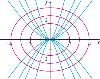
Consider the one-parameter family of circles \[ \begin{equation*} (x-1)^{2}+(y-2)^{2}=C\qquad C>0 \end{equation*} \]
with center at the point \((1,2)\) and radius \(\sqrt{C}\). Figure 1 shows some members of this family of circles. If the equation describing the circles is differentiated with respect to \(x\), we obtain \[ \begin{eqnarray*} 2(x-1)+2(y-2)y^{\prime} & =&0\\ y^{\prime} & =&-\frac{x-1}{y-2} \tag{1} \end{eqnarray*} \]
which represents the differential equation of the family of circles.
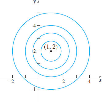
For a specific point \((x,y)\), \(y\neq 2\), on any one of the circles, the differential equation \(y^{\prime} =-\dfrac{x-1}{y-2}\) gives the slope of the tangent line at \((x,y)\).
Now let's consider another example. The family of nonvertical lines passing through the point \((1,2)\) satisfies the equation \[ \begin{equation*} y-2=m(x-1) \end{equation*} \]
1067
where \(m\) is the slope of a particular member of the family. The differential equation for this family of lines is \[ \begin{equation} y^{\prime} =m=\frac{y-2}{x-1} \tag{2} \end{equation} \]
Figure 2 shows some members of this family of lines.
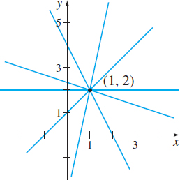
If we compare the differential equations (1) and (2), we see that the right side of (1) is the negative reciprocal of the right side of (2). From this, we conclude that if \((x,y)\) is a point of intersection of one of the circles and one of the lines from each family, then the line and the circle are perpendicular (orthogonal) to each other at the point of intersection. Each line in the family \(y-2=m(x-1)\) is an orthogonal trajectory of the family of circles, and conversely, each circle in the family \((x-1)^{2}+(y-2)^{2}=C\) is an orthogonal trajectory of the family of lines.
In general, if \(F(x,y,C)=0\) and \(G(x,y,K)=0\) are one-parameter families of curves, in which each member of one family intersects the members of the other family at a right angle, then the two families are said to be orthogonal trajectories of each other.
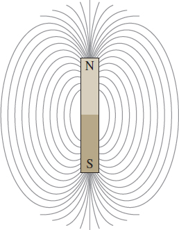
Orthogonal trajectories occur naturally. For example, iron filings sprinkled on a pane of glass over a bar magnet arrange themselves along a family of curved lines, indicating the direction of magnetic force. A family of orthogonal trajectories can be determined by locating all the points in the plane of the glass with the same potential energy.
To find a family \(G(x,y,K)=0\) of orthogonal trajectories for a given family \(F(x,y,C)=0,\) we use the steps below:
Steps for Finding a Family of Orthogonal Trajectories
Step 1 Find the differential equation for the given family.
Step 2 Replace \(y^{\prime} \) in this differential equation by \(-\dfrac{1}{y^{\prime} };\) the resulting equation is the differential equation for the family of orthogonal trajectories.
Step 3 Find the solution of the differential equation obtained in Step 2.
Finding a Family of Orthogonal Trajectories
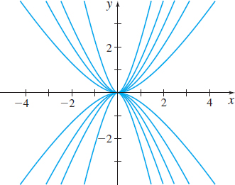
Find the family of orthogonal trajectories for the one-parameter family \(y^{2}=Cx^{3}\). See Figure 3 for several graphs in the family.
Solution
Step 1 We differentiate \(y^{2}=Cx^{3}\) with respect to \(x\). \[ 2yy^{\prime} =3Cx^{2} \]
Then we eliminate \(C\) using this equation and the equation \(y^{2}=Cx^{3}\) of the family. Since \(C=\dfrac{y^{2}}{x^{3}},\) we find \[ \begin{eqnarray*} 2yy^{\prime} & =&3\frac{y^{2}}{x^{3}}x^{2} \\ y^{\prime} & =&\frac{3y}{2x} \end{eqnarray*} \]
Step 2 Now we replace \(y^{\prime} \) with \(-\dfrac{1}{y^{\prime} },\) to obtain the differential equation for the family of orthogonal trajectories. \[ \begin{eqnarray*} -\dfrac{1}{y^{\prime} }& =&\frac{3y}{2x} \\ y^{\prime} & =&-\frac{2x}{3y} \end{eqnarray*} \]
1068
Blue: \(y^{2}=Cx^{3};\)
Pink: \(x^{2}+\dfrac{3}{2}y^{2}=k\)
Step 3 The differential equation \(\dfrac{dy}{dx}=-\dfrac{2x}{3y}\) is separable and can be written as \[ \begin{equation*} 2x\,dx+3y\,dy=0 \end{equation*} \]
The general solution is \[ \begin{equation*} x^{2}+\frac{3}{2}y^{2}=K \end{equation*} \]
The orthogonal trajectories for the family \(y^{2}=Cx^{3}\) is a family of ellipses \(x^{2}+\dfrac{3}{2}y^{2}=K\), as shown in Figure 4.
NOW WORK
Problem 43.
Inhibited Growth and Decay
Functions \(A=A( t) \), whose rates of change are \(\dfrac{{\it dA}}{dt}=kA\) , are said to follow the exponential law, or the law of uninhibited growth or decay. These models, discussed in Chapter 5, are examples of first-order differentiable equations. There, we found that the particular solution of \[ \begin{equation*} \dfrac{{\it dA}}{dt}=kA\qquad A( 0) =A_{0}>0 \end{equation*} \]
is \[ A(t)=A_{0}e^{kt} \]
NEED TO REVIEW?
Differential equations of the form \(\dfrac{{\it dA}}{dt}=kA\) are discussed in Section 5.5, pp. 382-384.
Notice that \[ \begin{equation*} \hbox{if}\qquad k>0,\qquad \lim_{t\rightarrow \infty }A(t)=\lim_{t\rightarrow \infty }\big( A_{0}e^{kt}\big) =\infty \quad \end{equation*} \]
which represents uninhibited growth, and \[ \begin{equation*} \hbox{if}\qquad k<0,\qquad \lim_{t\rightarrow \infty }A(t)=\lim_{t\rightarrow \infty }\big( A_{0}e^{kt}\big) =0\quad \end{equation*} \]
which represents uninhibited decay.
In contrast to uninhibited growth or decay, there are many situations in which the growth or decay is inhibited, that is, it is limited by some factor. For example, a new company entering a market in which the total sales in the market is $\(M\) might expect its annual sales to grow, but the sales can never exceed $\(M\). A possible model for the company to use to predict the growth of its sales is to assume that the rate of growth is proportional to the difference between its sales at time \(t\) and the upper limit $\(M\). If \(y=y(t)\) denotes the sales at time \(t\), then this situation is modeled by \[ \begin{equation*} \bbox[5px, border:1px solid black, #F9F7ED]{\bbox[#FAF8ED,5pt] {\dfrac{dy}{dt}=k(M-y)}} \end{equation*} \tag{3} \]
where \(k\) is a positive constant. Solving the separable differential equation, we have \[ \begin{eqnarray*} \dfrac{dy}{M-y} &=&k\,dt \\ -\ln \vert M-y\vert &=&kt+C_{1} \\ M-y &=&e^{-( kt\,{+}\,C_{1}) }=e^{-C_{1}}e^{-kt}\qquad \color{#0066A7}{{y<M,\hbox{ so } M-y>0}} \end{eqnarray*} \]
The general solution is \[ \begin{equation*} y=y( t) =M+Ce^{-kt} \qquad \hbox{where}\qquad C=-e^{-C_{1}} \end{equation*} \]
If we assume that sales are initially $\(R,\) then \(y(0)=R\geq 0\). Using this initial condition, \(R=M+Ce^0\) so \(C=R-M\). A particular solution is \[\bbox[5px, border:1px solid black, #F9F7ED]{\bbox[#FAF8ED,5pt] {y(t)=M+(R-M)e^{-kt}\qquad k>0}} \]
1069
Figure 5 shows the graph of \(y=y( t) .\)
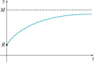
The function \(y=y(t)\) is increasing \([ y^{\prime} ( t) =k(M-y) >0] \), its graph is concave downward \([ y^{\prime \prime} ( t) =-ky^{\prime} ( t) <0] \), and \(\lim\limits_{t\rightarrow \infty }y(t)=M\). In the special case where \(R=0\), denoting that there are no sales when \(t=0,\) then \[ \begin{equation*} \bbox[5px, border:1px solid black, #F9F7ED]{\bbox[#FAF8ED,5pt] {y(t)=M( 1-e^{-kt})\qquad k>0}} \tag{4} \end{equation*} \]
Analyzing a Company 's Sales Growth
The annual sales of a new company are expected to grow at a rate proportional to the difference between the sales at time \(t\) and an upper limit of $\(5\) million. Suppose the sales are $0 initially and are $\(2\) million after \(4\) years of operation. Determine the annual sales at any time \(t\). How long will it take for the annual sales to reach $\(4\) million?
Solution Since there are no sales initially (\(R=0\)), we use equation (4). Then since the upper limit of sales is $\(5\) million, the sales at time \(t\) are \[ \begin{equation*} y(t)=5(1-e^{-kt})\qquad \color{#0066A7}{{M=5}} \end{equation*} \]
Since sales are $\(2\) million after \(4\) years, the boundary condition is \(y(4)=2.\) We use the boundary condition to find the constant \(k\): \[ \begin{eqnarray*} 2& =&5(1-e^{-4k})\qquad \color{#0066A7}{{y(4)=2}}\\ 5e^{-4k}& =&3 \\[2pt] e^{-4k}& =&0.6 \\[4pt] k& =&\frac{\ln 0.6}{-4} = -0.25\ln 0.6 \end{eqnarray*} \]
So, the function \[ \begin{equation*} y(t)=5\big(1-e^{( 0.25\ln 0.6) t}\big) \end{equation*} \]
models the company's sales in year \(t.\)
To find out how long it will take for sales to reach $\(4\) million, we solve the equation \(y( t) =4.\) Then \[ \begin{eqnarray*} 4& =&5\big( 1-e^{( 0.25\ln 0.6) t}\big) \\ 5e^{( 0.25\ln 0.6) t}& =&1 \\[1pt] (0.25\ln 0.6) t & =&\ln 0.2 \\[3pt] t& =&\frac{\ln 0.2}{0.25\ln 0.6}\approx 12.6 \hbox{years} \end{eqnarray*} \]
It will take approximately \(12.6\) years for annual sales to reach $\(4\) million.
The differential equation \(\dfrac{dy}{dt}=k(M-y),\) \(k>0,\) also models Newton's Law of Heating, where \(y(t)\) denotes the temperature of an object at time \(t\) units after it is placed in a warmer surrounding medium that is at the constant temperature \(M\).* The temperature of the object will never exceed \(M\).
*See Newton's Law of Cooling, which is discussed in Section 5.6, pp. 394-395.
NOW WORK
Problem 53.
The differential equation (3) is used to model productivity based on learning theory. Learning theory proposes that the time or effort needed to learn a specific repetitive skill decreases as the number of repetitions increases. In a paper published in the Journal of Aeronautical Science (February 1936), an aeronautical engineer Theodore P. Wright (1895–1970) applied learning theory to the repetitive work performed on an airplane assembly line. He developed a mathematical model, called a learning curve, to model employee productivity. This model is still used to obtain cost estimates.
1070
For example, suppose a new employee is hired to assemble a component of an airplane wing. If she needs to be trained before starting the job, then her productivity will follow a learning curve. If \(y=y( t) \) denotes the number of components assembled at time \(t,\) then her rate of productivity is modeled by the differential equation \[ \dfrac{dy}{dt}=k( M-y) \]
where \(k\) is a positive constant and the number of components she assembles per unit of time is limited by outside constraints to \(M\) units. Then, solving the differential equation, the assembler's productivity at time \(t\) is given by \[ y( t) =M( 1-e^{-kt}) \]
NOW WORK
Problem 55.