16.4 First-Order Linear Differential Equations; Bernoulli Differential Equations
OBJECTIVES
When you finish this section, you should be able to:
- Solve a first-order linear differential equation (p. 1078)
- Solve applied problems involving first-order linear differential equations (p. 1079)
- Find the general solution of a Bernoulli equation (p. 1082)
- Solve applied problems (p. 1083)
In this section, we solve first-order linear differential equations and Bernoulli differential equations. These differential equations occur in the study of free fall with air resistance, flow rates in mixtures, and logistic equations.
1 Solve a First-Order Linear Differential Equation
1078
We use integrating factors to solve first-order linear differential equations. Recall that a first-order differential equation is linear if it can be written in the form \[\bbox[5px, border:1px solid black, #F9F7ED]{\bbox[#FAF8ED,5pt] {\dfrac{dy}{dx}+P(x)\,y=Q(x)}} \tag{1} \]
where the functions \(P\) and \(Q\) are continuous on their domains.
For example, the differential equation \[ \frac{dy}{dx}-\frac{3}{x}y=x^{2} \]
is a first-order linear differential equation.
In the differential equation (1), either \(Q( x) =0\) or \(Q( x) \neq 0\). If \(Q( x) =0\), then \(\dfrac{dy}{dx}+P( x) y=0\), and the differential equation is separable: \[\bbox[5px, border:1px solid black, #F9F7ED]{\bbox[#FAF8ED,5pt] {\dfrac{dy}{y}+P(x)\,dx=0}} \]
The general solution of this differential equation is \[\bbox[5px, border:1px solid black, #F9F7ED]{\bbox[#FAF8ED,5pt] {\ln \left\vert y\right\vert + \int \!P(x)\,dx=C}} \]
NOW WORK
Problem 5.
If \(Q(x)\neq 0\), we solve (1) by multiplying by the integrating factor \[\bbox[5px, border:1px solid black, #F9F7ED]{\bbox[#FAF8ED,5pt]{ e^{\int P(x)\,dx} = \exp\left[\int P(x)\,dx\right] }} \] \[ \begin{eqnarray*} \dfrac{dy}{dx}+P(x)\,y &=&Q(x) \qquad\qquad\quad {\color{#0066A7}{\hbox{Equation (1)}, Q(x) \neq 0.}} \\ \frac{dy}{dx}e^{\int \!P(x)\,dx}+P(x)ye^{\int \!P(x)\,dx} &=&Q(x)e^{\int \!P(x)\,dx} \qquad {\color{#0066A7}{\hbox{Multiply (1) by exp }\left[\int \!P(x)\,dx\right].}} \end{eqnarray*} \]
The left side of this equation equals \(\dfrac{d}{dx}\!\left( y\cdot e^{\int \!P(x)\,dx}\right) \), so \[ \begin{equation*} \frac{d}{dx}\!\left( y\cdot e^{\int \!P(x)\,dx}\right) =Q(x)e^{\int \!P(x)\,dx} \end{equation*} \]
Now we integrate to obtain \[ \begin{equation*} {y\cdot e^{\int \!P(x)\,dx}=\int Q(x)e^{\int \!P(x)\,dx}dx+C} \tag{2} \end{equation*} \]
The general solution of the differential equation \(\dfrac{dy}{dx} +P(x)\,y=Q(x)\), \(Q( x) \neq 0\), is found by finding the integrals in (2) and solving for \(y\).
Solving a First-Order Linear Differential Equation
Find the general solution of the first-order linear differential equation \[ \frac{dy}{dx}+\frac{x}{x^{2}+1}y=\dfrac{x^{3}}{1+x^{2}} \]
Solution Compare the differential equation to (1). Since \(P(x)= \dfrac{x}{x^{2}+1}\), the integrating factor is \[ \begin{equation*} e^{\int \!P( x)\,dx} = \exp\; \left[{\int {\frac{x}{x^{2}+1}}\,dx}\right]= \exp \left[{\frac{1}{2} \ln ( x^{2}+1) }\right] = \exp\; \Big[{\ln ( x^{2}+1) ^{1/2}}\Big]= \sqrt{x^{2}+1} \end{equation*} \]
1079
Now we multiply the differential equation by \(\sqrt{x^{2}+1}\) and obtain \[ \begin{equation*} \sqrt{x^{2}+1}\,\frac{dy}{dx}+\dfrac{x}{\sqrt{x^{2}+1}}y=\dfrac{x^{3}}{\sqrt{ x^{2}+1}} \end{equation*} \]
The left side of the above equation is the derivative of \(\sqrt{x^{2}+1}\,y\), so we can write \[ \begin{equation*} \dfrac{d}{dx}\big( \sqrt{x^{2}+1}\,y\big) =\dfrac{x^{3}}{\sqrt{x^{2}+1}} \end{equation*} \]
Integrating both sides, we find \[ \begin{eqnarray*} \sqrt{x^{2}+1}\,y &=&\int \dfrac{x^{3}}{\sqrt{x^{2}+1}}\,dx \underset{\color{#0066A7}{\textrm{Let} \,u\,=\,x^{2}+1,\,du\,=\,2x\,dx}}{\underset{\color{#0066A7}\uparrow }{=}} \dfrac{1}{2}\int \dfrac{ \left( u-1\right) }{\sqrt{u}}\,du=\dfrac{1}{2}\int \big( {u^{1/2}}- {u^{-1/2}}\big)\,du \\ &=&\dfrac{1}{2}\left( \dfrac{u^{3/2}}{\dfrac{3}{2}}-\dfrac{u^{1/2}}{\dfrac{1 }{2}}\right) +C=\dfrac{( x^{2}+1) ^{3/2}}{3}-(x^{2}+1)^{1/2}+C \\ y &=&\dfrac{x^{2}+1}{3}-1+\dfrac{C}{\sqrt{x^{2}+1}}\qquad\color{#0066A7}{{\hbox{Solve for }y.}} \end{eqnarray*} \]
and we have the general solution to the differential equation.
NOW WORK
Problem 9.
2 Solve Applied Problems Involving First-Order Linear Differential Equations
Free Fall with Air Resistance
In Chapter 4, we saw that if air resistance is ignored, then the position \(s=s(t)\) at time \(t\) of an object with mass \(m\) in free fall obeys the equation \[ \begin{equation*} ma=-mg \end{equation*} \]
where \(a=\dfrac{d^{2}s}{dt^{2}}\) and \(g\) is the acceleration due to gravity.
A more realistic model of the motion of an object in free fall accounts for the effect of air resistance. A common assumption is that air resistance exerts a force proportional to the speed \(v\) of the object and opposite to the motion of the object. With this assumption, the motion of an object of mass \(m\) in free fall is described by the differential equation \[\bbox[5px, border:1px solid black, #F9F7ED]{\bbox[#FAF8ED,5pt] {m\dfrac{d^{2}s}{dt^{2}}=-mg-kv}} \]
where \(k>0\) is the constant of proportionality and depends on the particular object and certain air properties. For example, a sheet of paper has a much larger constant of proportionality than a solid lead ball has. Since \(v= \dfrac{ds}{dt}\), the second-order differential equation becomes \[ \begin{equation*} m\frac{dv}{dt}=-mg-kv \end{equation*} \] \[\bbox[5px, border:1px solid black, #F9F7ED]{\bbox[#FAF8ED,5pt] {\dfrac{dv}{dt}+\dfrac{k}{m}v=-g}} \]
1080
This is a first-order linear differential equation. To solve the differential equation, we multiply both sides by the integrating factor \(\exp \left[{\int {\dfrac{k}{m}\,dt}}\right]= \exp \left[{{\dfrac{k}{m}t}}\right]= e^{kt/m}\). \[ \begin{eqnarray*} e^{{{kt/m}}}\dfrac{dv}{dt}+e^{{{kt/m}}}\frac{k}{m} v &=&-g e^{{{kt/m}}} \\[4pt] \dfrac{d}{dt}\left[v e^{{{kt/m}}}\right] &=&-ge^{{{kt/m}}} \\ ve^{{{kt/m}}} &=&-g\int e^{{{kt/m}}}\, dt =-\dfrac{mg }{k}e^{{{kt/m}}}+C \quad\qquad\;\; \color{#0066A7}{\hbox{Integrate both sides.}} \\ v &=&\dfrac{-\dfrac{mg}{k}e^{{{kt/m}}}+C}{e^{{{kt/m}}}}=-\dfrac{mg}{k}+Ce^{{{-kt/m}}}\qquad\color{#0066A7}{\hbox{Solve for }v}. \end{eqnarray*} \]
The general solution is \[ \begin{equation*} v(t)=-\frac{mg}{k}+Ce^{{{-kt/m}}} \end{equation*} \]
If the object has initial velocity \(v_{0}\), then \[ \begin{equation*} v_{0}=v( 0) =-\frac{mg}{k}+C,\qquad\hbox{so}\qquad C=v_{0}+\dfrac{ mg}{k} \end{equation*} \]
Then \[ \begin{equation*} \bbox[5px, border:1px solid black, #F9F7ED]{\bbox[#FAF8ED,5pt] {v(t)=-\dfrac{mg}{k}+\left( v_{0}+\dfrac{mg}{k}\right) e^{-kt/m}}} \tag{3} \end{equation*} \]
Notice that \(\lim\limits_{t\rightarrow \infty }v(t)=-\dfrac{mg}{k}\). That is, the limiting velocity of a freely falling object depends only on the mass of the body and the constant of proportionality \(k\).
Solving a Free Fall Problem
A parachuter and his parachute together weigh \(192 {\rm lb}\). At the instant the parachute opens, he is falling at 150 feet per second (ft/s). Suppose the air resistance exerts a force of 200 lb when the parachuter’s speed is 20 ft/s.
- How fast is he falling \(3\) seconds after the parachute opens?
- What is the parachuter’s limiting velocity?
Solution (a) In the U.S. customary system of units, length is measured in feet, weight in pounds, time in seconds, and \(g\approx 32\;\rm{ft}/\rm{s}^{2}\). The mass \(m\) of the parachuter and his parachute obeys \(mg=\hbox{weight}=192\;\rm{lb}\).
NOTE
Remember that with falling objects, the positive direction is up, so \(v_0 = v(0) =-150\;\rm{ft}/\!\rm{s}\).
Since the air resistance is \(200\;\rm{lb}\) when the speed is \(20\;\rm{ft}/\rm{s}\), \[ \begin{eqnarray*} 200& =&k\cdot 20\qquad\color{#0066A7}{{F=kv}; \hbox{force is proportional to speed.}} \\ k& =&10 \end{eqnarray*} \]
From (3), the velocity of the parachuter at time \(t\) after the parachute opens is \[ \begin{eqnarray*} v(t) &=&-\frac{mg}{k}+\left( v_{0}+\frac{mg}{k}\right) e^{{{-kt/m}}} \\ v(t) &=&-\frac{192}{10}+\left( -150+\frac{192}{10}\right) e^{{{-10t/6}}}\qquad\color{#0066A7}{{v}_{0}=-150; mg=192; g=32; k=10.} \\ v(t) &=&-19.2-130.8e^{{{-5t/3}}} \end{eqnarray*} \]
1081
After \(3\) seconds, the parachuter’s velocity is \[ \begin{equation*} v(3)=-19.2-130.8e^{-5}\approx -20.081\;\rm{ft}/\!\rm{s} (13.692 \;\rm{mi}/\!\rm{h}) \end{equation*} \]
(b) The limiting velocity is \(\lim\limits_{t\rightarrow \infty }v(t)=-\dfrac{mg}{k}=-19.2\;\rm{ft}/\rm{s} (13.091\;\rm{mi}/\rm{h} )\).
NOW WORK
Problem 47.
Flow Rate in Mixtures
Solving a Flow Rate Problem
A large tank contains \(81\;\rm{gal}\) of brine in which \(20\;\rm{lb}\) of salt are dissolved. Brine containing \(3\;\rm{lb}\) of dissolved salt per gallon runs into the tank at the rate of \(5\;\rm{gal}/\rm{min}\). The mixture, kept uniform by stirring, drains from the tank at the rate of \(2 \;\rm{gal}/\rm{min}\). How much salt is in the tank at the end of \(37 \;\rm{min}\)? See Figure 6.
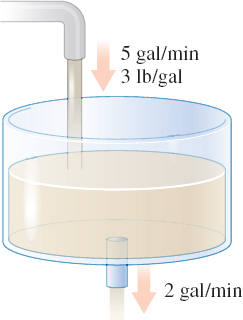
Solution Let \(y(t)\) be the amount of salt in the tank at time \(t\) . The rate of change \(\dfrac{dy}{dt}\) of salt in the tank at time \(t\) is the rate at which salt enters the tank minus the rate at which salt leaves the tank. Salt enters the tank at the rate of \(\left( 3\;\rm{lb}/\rm{gal}\right) \left(5\;\rm{gal}/\rm{min}\right) =15\;\rm{lb}/\rm{min}\).
To find the rate at which the salt exits the tank, we first need to find the concentration of salt in pounds per gallon at time \(t\). \[ \begin{equation*} \hbox{Concentration}=\dfrac{\hbox{amount of salt}}{\hbox{number of gallons}}= \frac{y(t)}{81+(5-2)t}=\dfrac{y( t) }{81+3t}\;\rm{lb}/\rm{gal} \end{equation*} \]
Then the rate at which the salt exits the tank is \[ \begin{equation*} \left( \dfrac{y( t) }{81+3t}\;\rm{lb}/\rm{gal}\right) \left( 2 \;\rm{gal}/\rm{min}\right) =\dfrac{2y( t) }{81+3t}\;\rm{lb}/\rm{min} \end{equation*} \]
The mixture problem is modeled by the differential equation \[ \begin{eqnarray*} \dfrac{dy}{dt}=\hbox{rate in }-\hbox{rate out}&=&15-\frac{2y( t) }{ 81+3t}\\ \dfrac{dy}{dt}+\frac{2}{3( 27+t) }y&=&15 \end{eqnarray*} \]
This is a first-order linear differential equation. We use the integrating factor: \[ \begin{eqnarray*} e^{\int \!P( t)\,dt}&=&\exp \!\left[ \int \!\dfrac{2}{3( 27+t) } dt\right] =\exp \!\left[ \dfrac{2}{3}\ln ( 27+t) \right]\\ &=&\exp\,[ \ln ( 27+t) ^{2/3}] =(27+t)^{2/3} \end{eqnarray*} \]
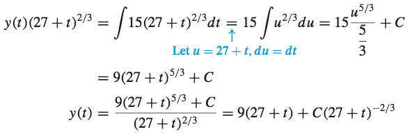
We multiply the differential equation by the integrating factor to obtain \[ \begin{eqnarray*} (27+t)^{2/3}\dfrac{dy}{dt}+\dfrac{2y}{3( 27+t) ^{1/3}} &=&15(27+t)^{2/3} \\ \frac{d}{dt}[y(t)(27+t)^{2/3}] &=&15(27+t)^{2/3} \end{eqnarray*} \]
Now we integrate both sides with respect to \(t\).
1082
Next we use the initial condition that \(y( 0) =20\;\rm{lb}\). Then \[ \begin{eqnarray*} y( 0) &=&20=9(27)+C(27)^{-2/3}\\ -223 &=&\dfrac{C}{9} \\ C &=&-2007 \end{eqnarray*} \]
The amount of salt \(y( t) \) in the brine at time \(t\) min is \[ \begin{equation*} y(t)=9(27+t)-2007(27+t)^{-2/3} \end{equation*} \]
The amount of salt in the tank at the end of \(37\;\rm{min}\) is \[ y(37)=9(27+37)-2007(27+37)^{-2/3}\approx 451\;\rm{lb} \]
NOW WORK
Problem 49.
3 Find the General Solution of a Bernoulli Equation
The equation \[ \begin{equation*} \bbox[5px, border:1px solid black, #F9F7ED]{\bbox[#FAF8ED,5pt] {\dfrac{dy}{dx}+P(x)y=Q(x)y^{n}\qquad n\neq 0\quad n\neq 1}} \tag{4} \end{equation*} \]
where \(P\) and \(Q\) are functions of \(x\) only, is called a Bernoulli equation, named for Jakob Bernoulli who studied it in 1695.
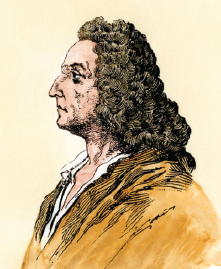
ORIGINS
Jakob (or James) Bernoulli (1654–1705) was a Swiss mathematician. Jakob was one of eight family members, in three generations of Bernoullis, who made major contributions to mathematics and physics.
If we multiply both sides of (3) by \(y^{-n}\) and make a judicious substitution, we obtain a first-order linear differential equation. First, we multiply (3) by \(y^{-n}\): \[ \begin{equation*} y^{-n}\frac{dy}{dx}+P(x)y^{-n+1}=Q(x) \tag{5} \end{equation*} \]
Now we use the substitution \(v=v( x) =y^{-n+1}\). Then \(\dfrac{dv}{ dx}=(1-n)y^{-n}\dfrac{dy}{dx}\). Since \(n\neq 0\) and \(n\neq 1\), we can write \(y^{-n}\dfrac{dy}{dx}=\dfrac{1}{1-n}\dfrac{dv}{dx}\). Then (4) becomes \[ \begin{eqnarray*} \frac{1}{1-n}\frac{dv}{dx}+P(x)v &=&Q(x) \\ \frac{dv}{dx}+(1-n)P(x)v &=&(1-n)Q(x) \qquad \color{#0066A7}{\hbox{Multiply by }1-n.} \end{eqnarray*} \]
This is a first-order linear differential equation in \(v=v( x) \).
We use the following steps to solve a Bernoulli equation:
Steps for Solving a Bernoulli Equation
\[ \dfrac{dy}{dx}+P(x)y=Q(x)y^{n}\qquad n\neq 0\quad n\neq 1 \]
Step 1 Multiply both sides of the equation by \(y^{-n}\). [This isolates \(Q( x) \) on the right.]
Step 2 Let \(v=v( x) =y^{-n+1}\). Then \(\dfrac{dv}{dx}=(1-n)y^{-n}\dfrac{dy}{dx}\).
Step 3 Substitute \(v\) and \(\dfrac{1}{1-n}\dfrac{dv}{dx}\) into \(y^{-n}\dfrac{dy}{dx}+ P(x)y^{-n+1} =Q(x)\).
Step 4 Find the general solution of the resulting first-order linear differential equation.
Step 5 Rewrite the general solution in terms of the original variables \(x\) and \(y\).
1083
Solving a Bernoulli Equation
Find the general solution of the differential equation \[ \begin{equation*} \frac{dy}{dx}=4y+2e^{x}y^{1/2} \end{equation*} \]
Solution We begin by writing the equation in the form of (3): \[ \begin{equation*} \frac{dy}{dx}-4y=2e^{x}y^{1/2} \end{equation*} \]
This is a Bernoulli differential equation with \(P(x)=-4\), \(Q(x)=2e^{x}\), and \(n=\dfrac{1}{2}\). Then we follow the steps for solving a Bernoulli equation.
Step 1 Multiply the differential equation by \(y^{-1/2}\) to obtain \[ \begin{equation*} y^{-1/2}\frac{dy}{dx}-4y^{1/2}=2e^{x} \end{equation*} \]
Step 2 Let \(v=v( x) =y^{1/2}\). Then \(\dfrac{dv}{dx}= \dfrac{1}{2}y^{-1/2}\dfrac{dy}{dx}\).
Step 3 Substitute \(v\) and \(\dfrac{dv}{dx}\) into \(y^{-1/2}\dfrac{dy }{dx}-4y^{1/2}=2e^{x}\). \[ \begin{eqnarray*} 2\dfrac{dv}{dx}-4v& =&2e^{x} \\ \dfrac{dv}{dx}-2v& =&e^{x} \end{eqnarray*} \]
This is a first-order linear differential equation in \(x\) and \(v\).
Step 4 Multiply the differential equation by the integrating factor \(e^{\int -2\,dx}=e^{-2x}\). \[ \begin{eqnarray*} e^{-2x}\dfrac{dv}{dx}-2e^{-2x}v& =&e^{-x} \\ \dfrac{d}{dx}(e^{-2x}v)& =&e^{-x} \\ e^{-2x}v& =&\int e^{-x}dx=-e^{-x}+C\quad C > 0 \\ v& =&Ce^{2x}-e^{x} \end{eqnarray*} \]
Step 5 Using \(v=y^{1/2}\), we write the solution in terms of \(x\) and \(y\). \[ \begin{eqnarray*} y^{1/2}& =&Ce^{2x}-e^{x} \\ y& =&(Ce^{2x}-e^{x})^{2} \end{eqnarray*} \]
NOTE
Since \(e^{-2x} v + e^{-x} > 0\), then \(C > 0\).
NOW WORK
Problem 25.
4 Solve Applied Problems
Logistic Growth
In the mid-nineteenth century, the Belgian mathematical biologist Pierre F. Verhulst (1804–1849) used the differential equation \[\bbox[5px, border:1px solid black, #F9F7ED]{\bbox[#FAF8ED,5pt] {\dfrac{dy}{dt}=ky(M-y)}} \]
where \(k\) and \(M\) are positive constants, to predict the human population of various countries. Verhulst referred to the model as logistic growth. Because of this, the equation is known as the logistic differential equation and its solutions are called logistic functions.
1084
Rewrite the differential equation as \[\bbox[5px, border:1px solid black, #F9F7ED]{\bbox[#FAF8ED,5pt] {\dfrac{dy}{dt}=kMy-ky^{2}}} \]
where the first term on the right side, \(kMy\), is a growth term and the second term, \(-ky^{2}\), is an “inhibition” or “competition” term that impedes growth.
The logistic differential equation \(\dfrac{dy}{dt}=kMy-ky^{2}\) is a Bernoulli differential equation: \[ \begin{equation*} \dfrac{dy}{dt}-kMy=-ky^{2} \end{equation*} \]
where \(P( t) =-kM\), \(Q( t) =-k\), and \(n=2\). To solve it, we follow the steps for solving a Bernoulli equation.
Step 1 Multiply by \(y^{-n}=y^{-2}\). \[ \begin{equation*} y^{-2}\dfrac{dy}{dt}+( -kM) y^{-1}=-k \end{equation*} \]
Step 2 Let \(v=y^{-1}\). Then \(\dfrac{dv}{dt}=-y^{-2}\dfrac{dy}{dt}\).
Step 3 Substitute \(v\) and \(\dfrac{dv}{dt}\) into \(y^{-2}\dfrac{dy}{dt} -kMy^{-1}=-k\). \[ \begin{eqnarray*} -\dfrac{dv}{dt} -kM v &=&-k \\ \dfrac{dv}{dt}+kMv &=&k \end{eqnarray*} \]
Step 4 Multiply by the integrating factor \(e^{\int \!P( t)\,dt}=e^{\int kM\,dt}=e^{{kMt}}\). \[ \begin{eqnarray*} e^{{kMt}}\dfrac{dv}{dt}+e^{{kMt}}kMv &=&ke^{{kMt}}\\ \dfrac{d}{dt} [e^{{kMt}}v] &=&ke^{{kMt}} \\ e^{{kMt}}v &=&k\int e^{{kMt}}dt=\dfrac{1}{M}e^{{kMt}}+C \end{eqnarray*} \]
Step 5 Using \(v=y^{-1}\), we rewrite the solution in terms of \(y\). \[ \begin{eqnarray*} e^{{kMt}}\dfrac{1}{y} &=&\dfrac{1}{M}e^{{kMt}}+C\qquad \color{#0066A7}{v=y^{-1} =\tfrac{1}{y}} \\ y(t) &=&\dfrac{e^{{kMt}}}{\dfrac{1}{M}e^{{kMt}}+C}=\frac{ Me^{{kMt}}}{e^{{kMt}}+MC}=\dfrac{M}{1+MCe^{-{kMt}} } \end{eqnarray*} \]
If we assume that the initial condition is \(y(0)=R\), \(\ 0\leq R<M\), then \(R= \dfrac{M}{1+MC}\) or \(C=\dfrac{M-R}{RM}\) and \[\bbox[5px, border:1px solid black, #F9F7ED]{\bbox[#FAF8ED,5pt] {y(t)=\dfrac{RM}{R+(M-R)e^{-kMt}}}} \tag{6} \]
Equation (5) is called a logistic function.
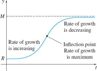
The graph of a logistic equation has a distinct “s” shape. See Figure 7. Since \(\lim\limits_{t\rightarrow \infty }y(t)=M\), \(M\) is called the carrying capacity of the logistic function.
Logistic equations have various applications:
- They are used to predict the growth of certain bacteria in a closed system where the scarcity of space or nutrients limits growth.
1085
- They provide a reasonable model for describing the spread of an epidemic caused by the introduction of an infected individual into a population. In this model, if \(M\) is the size of the population and \(y=y(t)\) is the number of infected individuals at time \(t\), then the logistic equation states that the spread (rate of growth) of the disease is proportional to the product of the number of infected individuals and the number of individuals who have not been infected. At the start of the epidemic, the disease spreads with uninhibited growth, and is modeled by the differential equation \(\dfrac{dy}{dt}=kMy\). See Section 5.5 for examples of uninhibited growth. Then since the number of individuals who are exposed is limited, at some point in time the rate of infection begins to decrease.
- In economics, the logistic equation is used to predict the growth of sales, the effects of advertising, and company growth. The logistic equation provides a reasonable model for describing the spread of a new technology. For example, after the introduction of the iPad®, the rate of sales increases rapidly for a time, until it reaches a maximum. Then although the sales continue to increase, the rate of sales begins to decrease.
- Social scientists use logistic equations to study cultural phenomena in a society. The 2011 Occupy Wall Street movement is one such example. On September 17, 2011, a small group of protestors gathered at Zuccotti Park in New York City to protest the high salaries of Wall Street executives. As the movement spread throughout the city and the United States, the number of protestors increased rapidly for a time, until reaching a maximum rate of increase. Then although more protestors joined the movement, the rate of increase began to decrease.
ORIGINS
Daniel Bernoulli (1700–1782) was the nephew of Jakob Bernoulli and son of mathematician Daniel Bernoulli. Daniel, the son, was a medical doctor and a mathematician who did much work with Leonhard Euler (1707–1783). In 1760 Daniel Bernoulli used what is now called the logistic equation to study the spread of smallpox.
Solving a Logistic Equation
An influenza epidemic is spreading throughout a population of \(50,000\) people at a rate that is proportional to the product of the number of infected people and the number of noninfected people. Suppose that \(100\) people were infected initially and \(1000\) were infected after \(10\) days.
- Find the number of infected people at any time \(t\). How long will it take for half the population to be infected?
- Find the time \(t\) at which the rate of spread of infection stops increasing and begins to decrease.
Solution (a) If \(y=y( t) \) is the number of people infected at time \(t\), then \[ \begin{equation*} \dfrac{dy}{dt}=ky( 50,000-y) \tag{7} \end{equation*} \]
where \(k\) is the constant of proportionality. As given in equation (5), the solution is \[ \begin{eqnarray*} y(t)&=&\frac{100(50,000)}{100+(50,000-100) e^{-50,000kt}}\qquad \color{#0066A7}{R=100,\quad M=50,000}\\ &=&\frac{100(50,000)}{100+49,900e^{-50,000kt}} =\frac{50,000}{1+499e^{-50,000kt}} \end{eqnarray*} \]
We find \(k\) from the boundary condition \(y(10)=1000\). Then \[ \begin{eqnarray*} 1000& =&\frac{50,000}{1+499e^{-500,000k}} \\ 499e^{-500,000k}& =&49 \\ -500,000k& =&\ln \left( \frac{49}{499}\right) \\ k& \approx &0.00000464=4.64 \times 10^{-6} \end{eqnarray*} \]
1086
So, \[ \begin{equation*} y(t)=\frac{50,000}{1+499e^{-0.232t}} \end{equation*} \]
Half the population is infected when \(y(t)=25,000\). \[ \begin{eqnarray*} 25,000& =&\dfrac{50,000}{1+499e^{-0.232t}} \\ 1+499e^{-0.232t}& =&2 \\ e^{-0.232t}& =&\frac{1}{499} \\ t& =&\frac{\ln \dfrac{1}{499}}{-0.232}\approx 27 \hbox{days} \end{eqnarray*} \]
Half the population is infected in approximately \(27\) days.
(b) The time \(t\) we seek is the inflection point of \(y=y( t) \). We need to find \(t\) so that \(y^{\prime \prime} ( t) =0\). \[ \begin{eqnarray*} y^{\prime} ( t) &=&ky( 50,000-y) =k( 50,000y-y^{2})\qquad \color{#0066A7}{{(6)}} \\ y^{\prime \prime} &=&k( 50,000y^{\prime} -2yy^{\prime} ) =0 \\ 2y &=&50,000 \\ y &=&25,000 \end{eqnarray*} \]
From (a), \(y=25,000\) when \(t=27\). That is, on Day \(27\), the rate of infection stops increasing and begins to decrease.
NOW WORK
Problem 51.