P.2 Library of Functions; Mathematical Modeling
OBJECTIVES
When you finish this section, you should be able to:
- Develop a library of functions (p. 15)
- Analyze a polynomial function and its graph (p. 17)
- Find the domain and the intercepts of a rational function (p. 19)
- Construct a mathematical model (p. 20)
When a collection of functions have common properties, they can be “grouped together" as belonging to a class of functions. Polynomial functions, exponential functions, and trigonometric functions are examples of classes of functions. As we investigate principles of calculus, we will find that often a principle applies to all functions in a class in the same way.
1 Develop a Library of Functions
15
Most of the functions in this section will be familiar to you; several might be new. Although the list may seem familiar, pay special attention to the domain of each function and to its properties, particularly to the shape of each graph. Knowing these graphs lays the foundation for later graphing techniques.
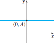
\[ {\bf Constant\;Function}\quad \quad \bbox[5px, border:1px solid black, #F9F7ED]{\bbox[#FAF8ED,5pt]{f ( x) =A}}\quad {A}~{\rm{is\;a\;real\;number}} \]
The domain of a constant function is the set of all real numbers; its range is the single number \(A\). The graph of a constant function is a horizontal line whose \(y\)-intercept is \(A;\) it has no \(x\)-intercept if \( A\neq 0\). A constant function is an even function. See Figure 18.
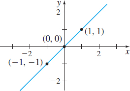
\[ {\bf {Identity\;Function}}\quad \quad \bbox[5px, border:1px solid black, #F9F7ED]{\bbox[#FAF8ED,5pt]{f( x) =x}} \]
The domain and the range of the identity function are the set of all real numbers. Its graph is the line through the origin whose slope is \( m=1\). Its only intercept is \(( 0,0)\). The identity function is an odd function; its graph is symmetric with respect to the origin. It is increasing over its domain. See Figure 19.
Notice that the graph of \(f(x)=x\) bisects quadrants I and III.
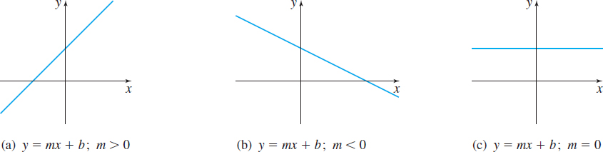
The graphs of both the constant function and the identity function are straight lines. These functions belong to the class of linear functions: \[{\bf {Linear\;Functions}}\quad \quad \bbox[5px, border:1px solid black, #F9F7ED]{\bbox[#FAF8ED,5pt]{f ( x) =mx+b}}\quad {m}\;{\rm{and}}\;{b}\;{\rm{are\;real\;numbers}}\]
NEED TO REVIEW?
Equations of lines are discussed in Appendix A.3, pp. A-18 to A-21.
The domain of a linear function is the set of all real numbers. The graph of a linear function is a line with slope \(m\) and \(y\)-intercept \(b\). If \(m>0\), \(f\) is an increasing function, and if \(m<0\), \(f\) is a decreasing function. If \(m=0\), then \(f\) is a constant function, and its graph is the horizontal line, \(y=b\). See Figure 20.
In a power function, the independent variable \(x\) is raised to a power. \[ {\bf{Power}}\;{\bf{Functions}}\quad \quad \bbox[5px, border:1px solid black, #F9F7ED]{\bbox[#FAF8ED,5pt]{f(x) = x^a}} \quad \quad a\;{\rm{is}}\;{\rm{a}}\;{\rm{real}}\;{\rm{number}} \]
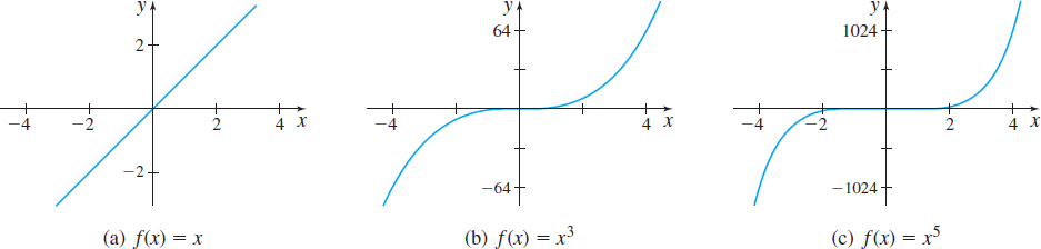
Below we examine power functions \(f( x) =x^{n},\) where \(n\geq 1\) is a positive integer. The domain of these power functions is the set of all real numbers. The only intercept of their graph is the point \(( 0,0) \).
If \(f\) is a power function and \(n\) is a positive odd integer, then \(f\) is an odd function whose range is the set of all real numbers and the graph of \(f\) is symmetric with respect to the origin. The points \(( -1,-1) \), \( ( 0,0) \), and \(( 1,1) \) are on the graph of \(f\). As \(x\) becomes unbounded in the negative direction, \(f\) also becomes unbounded in the negative direction. Similarly, as \(x\) becomes unbounded in the positive direction, \(f\) also becomes unbounded in the positive direction. The function \(f\) is increasing over its domain.
16
The graphs of several odd power functions are given in Figure 21.
If \(f\) is a power function and \(n\) is a positive even integer, then \(f\) is an even function whose range is \(\{ y|y\geq 0\}\). The graph of \(f\) is symmetric with respect to the \(y\)-axis. The points \(( -1,1) \), \(( 0,0) \), and \(( 1,1) \) are on the graph of \(f\). As \(x\) becomes unbounded in either the negative direction or the positive direction, \(f\) becomes unbounded in the positive direction. The function is decreasing on the interval \(( -\infty ,0] \) and is increasing on the interval \([ 0,\infty ) \).
The graphs of several even power functions are shown in Figure 22.
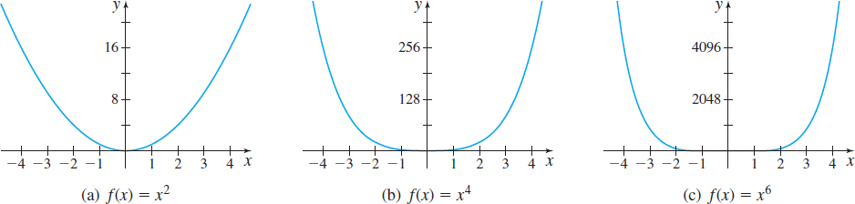
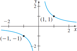
Look closely at Figures 21 and 22. As the integer exponent \(n\) increases, the graph of \(f\) is flatter (closer to the \(x\)-axis) when \(x\) is in the interval \(( -1,1) \) and steeper when \(x\) is in interval \( ( -\infty ,-1) \) or \((1,\infty )\). \[ {\bf{The}}\;{\bf{Reciprocal}}\;{\bf{Function}}\quad \quad \bbox[5px, border:1px solid black, #F9F7ED]{\bbox[#FAF8ED,5pt]{f(x) = \frac{1}{x}}} \]
The domain and the range of the reciprocal function (the power function \( f( x) =x^{a}\), \(a=-1\)) are the set of all nonzero real numbers. The graph has no intercepts. The reciprocal function is an odd function so the graph is symmetric with respect to the origin. The function is decreasing on \(( -\infty ,0) \) and on \(( 0,\infty ) \). See Figure 23.
\[ {\bf{Root}}\;{\bf{Functions}}\quad \quad \bbox[5px, border:1px solid black, #F9F7ED]{\bbox[#FAF8ED,5pt]{f(x) = x^{1/n} = \sqrt[n]{x}}}\quad n \ge 2\;{\rm{is}}\;{\rm{a}}\;{\rm{positive}}\;{\rm{integer}} \]
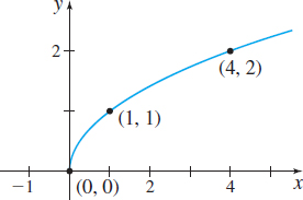
Root functions are also power functions. If \(n=2,\) \(f( x) =x^{1/2}= \sqrt{x}\) is the square root function. The domain and the range of the square root function are the set of nonnegative real numbers. The intercept is the point \(( 0,0)\). The square root function is neither even nor odd; it is increasing on the interval \([ 0,\infty ) \).
See Figure 24.
For root functions whose index \(n\) is a positive even integer, the domain and the range are the set of nonnegative real numbers. The intercept is the point \(( 0,0) .\) Such functions are neither even nor odd; they are increasing on their domain, the interval \([0,\infty )\).
If \(n=3,\) \(f( x) =x^{1/3}=\sqrt[{ 3}]{x}\) is the cube root function. The domain and range of the cube root function are all real numbers. The intercept of the graph of the cube root function is the point \(( 0,0) .\)
17
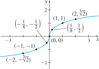
Because \(f( -x) =\sqrt[3]{-x}=-\sqrt[3]{x}=-f( x) ,\) the cube root function is odd. Its graph is symmetric with respect to the origin. The cube root function is increasing on the interval \(( -\infty ,\infty )\). See Figure 25.
For root functions whose index \(n\) is a positive odd integer, the domain and the range are the set of all real numbers. The intercept is the point \( ( 0,0) .\) Such functions are odd so their graphs are symmetric with respect to the origin. They are increasing on the interval \(( -\infty ,\infty )\). \[ {\bf{Absolute}}\;{\bf{value}}\;{\bf{Function}}\quad \quad \bbox[5px, border:1px solid black, #F9F7ED]{\bbox[#FAF8ED,5pt]{f(x) = |x|}} \]
The absolute value function is defined as the piecewise-defined function \[\bbox[5px, border:1px solid black, #F9F7ED]{\bbox[#FAF8ED,5pt]{\begin{array}{*{20}c} {f(x) = |x| = \left\{ {\begin{array}{*{20}c} x & {{\rm{if}}} & \;{x \ge {\rm{0}}} \\ { - x} & {{\rm{if}}} & \;{x\;{\rm{ < }}\;{\rm{0}}} \\ \end{array}} \right.} \\ \end{array}}} \]
or as the root function \[\bbox[5px, border:1px solid black, #F9F7ED]{\bbox[#FAF8ED,5pt]{f(x) = |x| = \sqrt {x^2 }}} \]
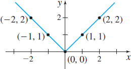
The domain of the absolute value function is the set of all real numbers. The range is the set of nonnegative real numbers. The intercept of the graph of \(f\) is the point \(( 0,0) .\) Because \(f ( -x ) = \vert {-}x \vert = \vert x \vert =f( x)\), the absolute value function is even. Its graph is symmetric with respect to the \( y\)-axis. See Figure 26.
NOW WORK
Problems 11 and 15.
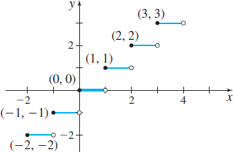
The floor function, also known as the greatest integer function, is defined as the largest integer less than or equal to \(x\): \[\bbox[5px, border:1px solid black, #F9F7ED]{\bbox[#FAF8ED,5pt]{f(x) = \left\lfloor x \right\rfloor = {\rm{largest}}\;{\rm{integer}}\;{\rm{less}}\;{\rm{than}}\;{\rm{or}}\;{\rm{equal}}\;{\rm{to}}\;x}} \]
The domain of the floor function \(\lfloor x\rfloor \) is the set of all real numbers; the range is the set of all integers. The \(y\)-intercept of \(\lfloor x\rfloor \) is \(0\), and the \(x\)-intercepts are the numbers in the interval \( [0,1).\) The floor function is constant on every interval of the form \( [k,k+1)\), where \(k\) is an integer, and is nondecreasing on its domain. See Figure 27.
IN WORDS
The floor function can be thought of as the “rounding down” function. The ceiling function can be thought of as the “rounding up” function.
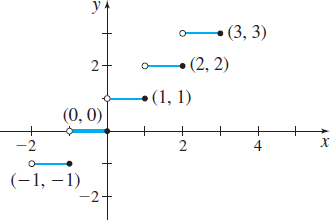
The ceiling function is defined as the smallest integer greater than or equal to \(x\): \[\bbox[5px, border:1px solid black, #F9F7ED]{\bbox[#FAF8ED,5pt]{f(x) = \left\lceil x \right\rceil = {\rm{smallest\;integer\;greater\;than\;or\;equal\;to}}\;x}} \]
The domain of the ceiling function \(\lceil x\rceil \) is the set of all real numbers; the range is the set of integers. The \(y\)-intercept of \(\lceil x\rceil \) is \(0\), and the \(x\)-intercepts are the numbers in the interval \( (-1,0].\) The ceiling function is constant on every interval of the form \( (k,\,k+1]\), where \(k\) is an integer, and is nondecreasing on its domain. See Figure 28.
For example, for the floor function \(\lfloor 5\rfloor =5\) and \(\lfloor 4.9\rfloor =4\), but for the ceiling function \(\lceil 5\rceil =5\) and \( \lceil 4.9\rceil =5.\)
The floor and ceiling functions are examples of step functions. At each integer the function has a discontinuity. That is, at integers the function jumps from one value to another without taking on any of the intermediate values.
2 Analyze a Polynomial Function and Its Graph
NOTE
![]() When graphing a function with a graphing utility, the option of using a connected mode or dot mode exists. When graphing the floor function and other functions with discontinuities, use dot mode to prevent the grapher from connecting the dots when \(f\) changes from one integer to the next.
When graphing a function with a graphing utility, the option of using a connected mode or dot mode exists. When graphing the floor function and other functions with discontinuities, use dot mode to prevent the grapher from connecting the dots when \(f\) changes from one integer to the next.
A monomial is a function of the form \(y=ax^{n},\) where \(a\neq 0\) is a real number and \(n\geq 0\) is an integer. Polynomial functions are formed by adding a finite number of monomials.
spanDEFINITIONspan Polynomial Function
A polynomial function is a function of the form \[\bbox[5px, border:1px solid black, #F9F7ED]{\bbox[#FAF8ED,5pt]{ f ( x ) =a_{n}x^{n}+a_{n-1}x^{n-1}+\cdots +a_{1}x+a_{0} }} \] where \(a_{n}\), \(a_{n-1}, \ldots , a_{1}\), \(a_{0}\) are real numbers and \(n\) is a nonnegative integer. The domain of a polynomial function is the set of all real numbers.
18
If \(a_{n}\neq 0\), then \(a_{n}\) is called the leading coefficient of \(f\), and the polynomial has degree \(n\).
The constant function \(f ( x ) =A\), where \(A\neq 0\), is a polynomial function of degree 0. The constant function \(f ( x ) =0 \) is the zero polynomial function and has no degree. Its graph is a horizontal line containing the point \(( 0,0) .\)
If the degree of a polynomial function is \(1\), then it is a linear function of the form \(f ( x ) =mx+b,\) where \(m\neq 0.\) The graph of a linear function is a straight line with slope \(m\) and \(y\)-intercept \(b\).
NEED TO REVIEW?
Quadratic equations and the discriminant are discussed in Appendix A.1, p. A-3.
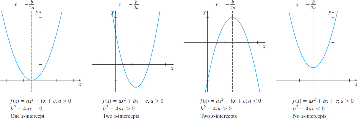
Any polynomial function \(f\) of degree \(2\) can be written in the form \[\bbox[5px, border:1px solid black, #F9F7ED]{\bbox[#FAF8ED,5pt]{f ( x ) =ax^{2}+bx+c}} \] where \(a\), \(b\), and \(c\) are constants and \(a\neq 0\). The square function \( f ( x ) =x^{2}\) is a polynomial function of degree \(2\). Polynomial functions of degree \(2\) are also called quadratic functions. The graph of a quadratic function is known as a parabola and is symmetric about its axis of symmetry, the vertical line \(x=-\dfrac{b }{2a}.\) Figure 29 shows the graphs of typical parabolas and their axis of symmetry. The \(x\)-intercepts, if any, of a quadratic function satisfy the quadratic equation \(ax^2+bx+c=0\).
Graphs of polynomial functions have many properties in common.
The zeros of a polynomial function \(f\) give insight into the graph of \(f\). If \(r\) is a real zero of a polynomial function \(f\), then \(r\) is an \(x\)-intercept of the graph of \(f,\) and \( ( x-r ) \) is a factor of \(f\).
NOTE
Finding the zeros of a polynomial function \(f\) is easy if \(f\) is linear, quadratic, or in factored form. Otherwise, finding the zeros can be difficult.
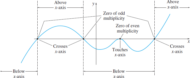
If \( ( x-r ) \) occurs more than once in the factored form of \(f\), then \(r\) is called a repeated or multiple zero of \(f\). In particular, if \( ( x-r ) ^{m}\) is a factor of \(f\), but \( ( x-r ) ^{m+1},\) where \(m\geq 1\) is an integer, is not a factor of \(f\), then \(r\) is called a zero of multiplicity \(m\) of \(f\). When the multiplicity of a zero \(r\) is an even integer, the graph of \(f\) will touch (but not cross) the \(x\)-axis at \(r\); when the multiplicity of \(r\) is an odd integer, then the graph of \(f\) will cross the \(x\)-axis at \(r\). See Figure 30 on page 19.
Analyzing the Graph of a Polynomial Function
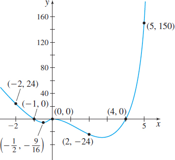
For the polynomial function \(f ( x ) =x^{2} ( x-4 ) ( x+1 ) \):
- Find the \(x\)- and \(y\)-intercepts of the graph of \(f\).
- Determine whether the graph crosses or touches the \(x\)-axis at each \(x\)-intercept.
- Plot at least one point to the left and right of each \(x\)-intercept and connect the points to obtain the graph.
19
Solution
- The \(y\)-intercept is \(f ( 0 ) =0.\) The \(x\)-intercepts are the zeros of the function: \(0\), \(4\), and \(-1\).
- \(0\) is a zero of multiplicity \(2\); the graph of \(f\) will touch the \(x\)-axis at \(0\). The numbers \(4\) and \(-1\) are zeros of multiplicity \(1\); the graph of \(f\) will cross the \(x\)-axis at \(4\) and \(-1\).
- Since \(f ( -2 ) =24\), \(f \!\left( -\dfrac{1}{2} \right) =-\dfrac{9}{16}\), \(f ( 2 ) =-24\), and \(f ( 5 ) =150,\) the points \( ( -2,24 )\), \(\left( -\dfrac{1}{2},-\dfrac{9}{16} \right) \), \( ( 2,-24 )\), and \( ( 5,150 ) \) are on the graph. See Figure 31.
NOW WORK
Problem 21.
3 Find the Domain and the Intercepts of a Rational Function
The quotient of two polynomial functions \(p\) and \(q\) is called a rational function.
spanDEFINITIONspan Rational Function
A rational function is a function of the form \[\bbox[5px, border:1px solid black, #F9F7ED]{\bbox[#FAF8ED,5pt]{ R ( x ) =\dfrac{p ( x ) }{q ( x ) } }} \] where \(p\) and \(q\) are polynomial functions and \(q\) is not the zero polynomial. The domain of \(R\) is the set of all real numbers, except those for which the denominator \(q\) is \(0\).
If \(R( x) =\dfrac{p( x) }{q( x) }\) is a rational function, the real zeros, if any, of the numerator, which are also in the domain of \(R\), are the \(x\)-intercepts of the graph of \(R\).

Finding the Domain and the Intercepts of a Rational Function
Find the domain and the intercepts (if any) of each rational function:
- \(R( x) =\dfrac{2x^{2}-4}{x^{2}-4}\)
- \(R( x) =\dfrac{x}{x^{2}+1}\)
- \(R(x) =\dfrac{x^{2}-1}{x-1}\)
Solution
- The domain of \(R ( x) =\dfrac{2x^{2}-4}{ x^{2}-4}\) is \( \{ x|x\neq -2;x\neq 2\}\). Since \(0\) is in the domain of \(R\) and \(R ( 0) =1\), the \(y\)-intercept is \(1\). The zeros of \(R\) are solutions of the equation \(2x^{2}-4=0\) or \(x^{2}=2.\) Since \(- \sqrt{2}\) and \( \sqrt{2}\) are in the domain of \(R,\) the \(x\)-intercepts are \(- \sqrt{2}\) and \( \sqrt{2}\).
- The domain of \(R ( x) =\dfrac{x}{x^{2}+1}\) is the set of all real numbers. Since \(0\) is in the domain of \(R\) and \(R ( 0) =0,\) the \(y\)-intercept is \(0\), and the \(x\)-intercept is also \(0\).
- The domain of \(R ( x) =\dfrac{x^{2}-1}{x-1}\) is \( \{ x|x\neq 1\}\). Since \(0\) is in the domain of \(R\) and \( R ( 0) =1\), the \(y\)-intercept is \(1\). The \(x\)-intercept(s), if any, satisfy the equation \begin{eqnarray*} x^{2}-1 &=&0 \\[0pt] x^{2} &=&1 \\[0pt] x &=&-1\quad\hbox{or}\quad x=1 \end{eqnarray*} Since \(1\) is not in the domain of \(R,\) the only \(x\)-intercept is \(-1\).
20
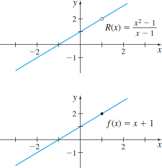
Figure 32 shows the graphs of \(R ( x) =\dfrac{x^{2}-1}{x-1}\) and \( f ( x) =x+1.\) Notice the “hole” in the graph of \(R\) at the point \( ( 1,2) .\) Also, \(R ( x) =\dfrac{x^{2}-1}{x-1}\) and \(f ( x) =x+1\) are not the same function: their domains are different. The domain of \(R\) is \(\{ x|x\neq 1\}\) and the domain of \(f\) is the set of all real numbers.
NOW WORK
Problem 27.
Algebraic Functions
Every function discussed so far belongs to a broad class of functions called algebraic functions. A function \(f\) is called algebraic if it can be expressed in terms of sums, differences, products, quotients, powers, or roots of polynomial functions. For example, the function \(f\) defined by \[ f( x) =\dfrac{3x^{3}-x^{2}( x+1) ^{4/3}}{ \sqrt{x^{4}+2}} \] is an algebraic function. Functions that are not algebraic are called transcendental functions. Examples of transcendental functions include the trigonometric functions, exponential functions, and logarithmic functions, which are discussed in the later sections of this chapter.
4 Construct a Mathematical Model
Problems in engineering and the sciences often can by solved using mathematical models that involve functions. To build a model, verbal descriptions must be translated into the language of mathematics by assigning symbols to represent the independent and dependent variables and then finding a function that relates the variables.
Constructing a Model from a Verbal Description
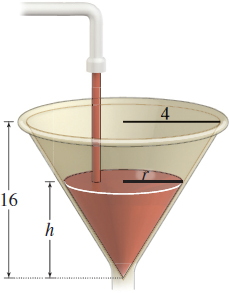
A liquid is poured into a container in the shape of a right circular cone with radius 4 meters and height 16 meters, as shown in Figure 33. Express the volume \(V\) of the liquid as a function of the height \(h\) of the liquid.
Solution The formula for the volume of a right circular cone of radius \(r\) and height \(h\) is \[ V=\dfrac{1}{3}\pi r^{2}h \]
The volume depends on two variables, \(r\) and \(h\). To express \(V\) as a function of \(h\) only, we use the fact that a cross section of the cone and the liquid form two similar triangles. See Figure 34.
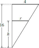
Corresponding sides of similar triangles are in proportion. Since the cone's radius is 4 meters and its height is 16 meters, we have \begin{eqnarray*} \dfrac{r}{h} &=&\dfrac{4}{16}=\dfrac{1}{4} \\[4pt] r &=&\dfrac{1}{4}h \end{eqnarray*}
21
NEED TO REVIEW?
Similar triangles and geometry formulas are discussed in Appendix A.2, pp. A-13 to A-14.
Then \[ \begin{array}{l} V = \frac{1}{3}\pi r^2 h\mathop = \limits_ {\color{#0066A7}{\uparrow}} \frac{1}{3}\pi \left( {\frac{1}{4}h} \right)^2 h = \frac{1}{{48}}\pi h^3 \\ \quad \quad \quad \;\;\;{\color{#0066A7}{r = \;\frac{1}{4}h}} \\ \end{array} \]
So \(V=V( h) =\dfrac{1}{48}\pi h^{3}\) expresses the volume \(V\) as a function of the height of the liquid. Since \(h\) is measured in meters, \(V\) will be expressed in cubic meters.
NOW WORK
Problem 29.
In many applications, data are collected and are used to build the mathematical model. If the data involve two variables, the first step is to plot ordered pairs using rectangular coordinates. The resulting graph is called a scatter plot.
Scatter plots are used to help suggest the type of relation that exists between the two variables. Once the general shape of the relation is recognized, a function can be chosen whose graph closely resembles the shape in the scatter plot.
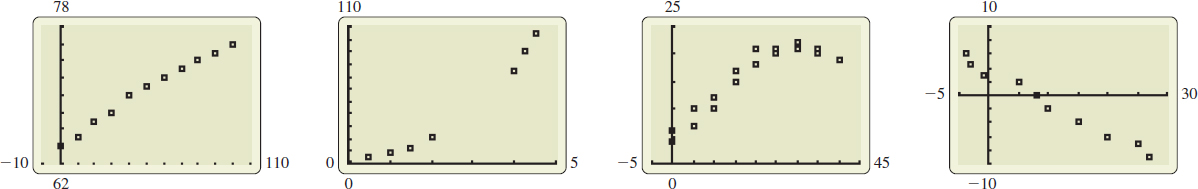
Identifying the Shape of a Scatter Plot
Determine whether you would model the relation between the two variables shown in each scatter plot in Figure 35 with a linear function or a quadratic function.
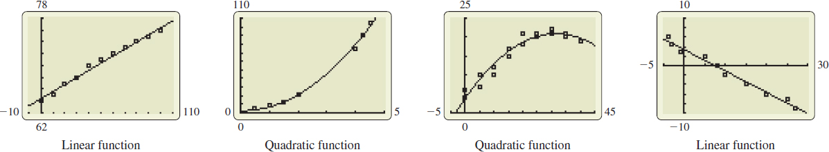
Solution For each scatter plot, we choose a function whose graph closely resembles the shape of the scatter plot. See Figure 36.
| Plot | Fertilizer, \(x\) (Pounds/\(100 \text{ft}^{2}\)) | Yield (Bushels) |
|---|---|---|
| 1 | 0 | 4 |
| 2 | 0 | 6 |
| 3 | 5 | 10 |
| 4 | 5 | 7 |
| 5 | 10 | 12 |
| 6 | 10 | 10 |
| 7 | 15 | 15 |
| 8 | 15 | 17 |
| 9 | 20 | 18 |
| 10 | 20 | 21 |
| 11 | 25 | 20 |
| 12 | 25 | 21 |
| 13 | 30 | 21 |
| 14 | 30 | 22 |
| 15 | 35 | 21 |
| 16 | 35 | 20 |
| 17 | 40 | 19 |
| 18 | 40 | 19 |
Building a Function from Data
![]() The data shown in Table 3 measure crop yield for various amounts of fertilizer:
The data shown in Table 3 measure crop yield for various amounts of fertilizer:
- Draw a scatter plot of the data and determine a possible type of relation that may exist between the two variables.
- Use technology to find the function of best fit to these data.
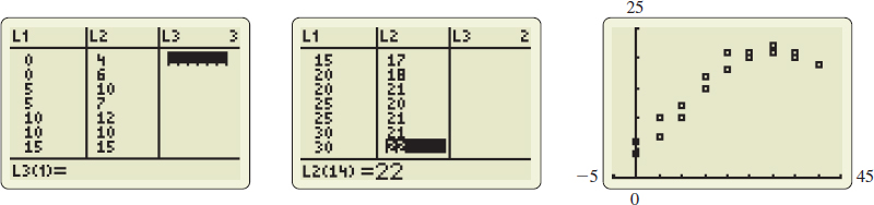
Solution (a) Figure 37 on page 22 shows the scatter plot. The data suggest the graph of a quadratic function.
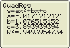
(b) The graphing calculator screen in Figure 38 shows that the quadratic function of best fit is \[ Y ( x) =-0.017x^{2}+1.0765x+3.8939 \] where \(x\) represents the amount of fertilizer used and \(Y\) represents crop yield. The graph of the quadratic model is illustrated in Figure 39.
22

NOW WORK
Problem 31.