4.6 Using Calculus to Graph Functions
308
OBJECTIVES
When you finish this section, you should be able to:
- Graph a function using calculus (p. 308)
In precalculus, algebra was used to graph a function. In this section, we combine precalculus methods with differential calculus to obtain a more detailed graph.
1 Graph a Function Using Calculus
The following steps are used to graph a function by hand or to analyze a computer-generated graph of a function.
Steps for Graphing a Function \({y=f(x)}\)
Step 1 Find the domain of \(f\) and any intercepts.
Step 2 Identify any asymptotes, and examine the end behavior.
Step 3 Find \(y^\prime =f^\prime (x)\) and use it to find any critical numbers of \(f.\) Determine the slope of the tangent line at the critical numbers. Also find \(f^{\prime \prime} .\)
Step 4 Use the Increasing/Decreasing Function Test to identify intervals on which \(f\) is increasing \((f^\prime >0)\) and the intervals on which \(f\) is decreasing \((f^\prime <0)\).
Step 5 Use either the First Derivative Test or the Second Derivative Test (if applicable) to identify local maximum values and local minimum values.
Step 6 Use the Test for Concavity to determine intervals where the function is concave up \((f^{\prime \prime} >0)\) and concave down \((f^{\prime \prime} <0)\). Identify any inflection points.
Step 7 Graph the function using the information gathered. Plot additional points as needed. It may be helpful to find the value of the derivative at such points.

Using Calculus to Graph a Polynomial Function
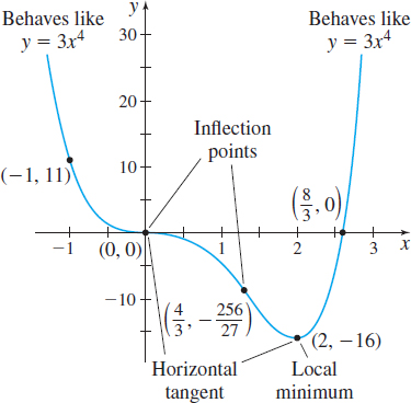
Graph \(f(x)=3x^{4}-8x^{3}\).
Solution We follow the steps for graphing a function.
Step 1 \(f\) is a fourth-degree polynomial; its domain is all real numbers. \(f( 0) =0\), so the \(y\)-intercept is \(0\). We find the \(x\)-intercepts by solving \(f(x) =0\). \[ \begin{eqnarray*} 3x^{4}-8x^{3} &=&0 \\ x^{3}( 3x-8) &=&0 \\ x &=&0 \qquad\hbox{or}\qquad x=\dfrac{8}{3} \end{eqnarray*} \]
There are two \(x\)-intercepts: \(0\) and \(\dfrac{8}{3}\). We plot the intercepts \((0,0)\) and \(\left( \dfrac{8}{3},0\right)\)
Step 2 Polynomials have no asymptotes, but the end behavior of \(f\) resembles the power function \(y=3x^{4}\).
Step 3 \(f^\prime (x) =12x^{3}-24x^{2}=12x^{2}(x-2)\qquad f^{\prime \prime} (x) =36x^{2}-48x=12x( 3x-4) \)
For polynomials, the critical numbers occur when \(f^\prime (x) =0\). \[ \begin{eqnarray*} 12x^{2}( x-2) &=&0 \\ x &=&0 \qquad \hbox{or}\qquad x=2 \end{eqnarray*} \]
NOTE
When graphing a function, piece together a sketch of the graph as you go, to ensure that the information is consistent and makes sense. If it appears to be contradictory, check your work. You may have made an error.
The critical numbers are \(0\) and \(2\). At the points \((0,0)\) and \(( 2,-16)\) , the tangent lines are horizontal. We plot these points.
Step 4 To apply the Increasing/Decreasing Function Test, we use the critical numbers \(0\) and \(2\) to form three intervals.
309
| Interval | Sign of f\(^\prime (x)\) | Conclusion |
|---|---|---|
| \((-\infty ,0)\) | negative | \(f\) is decreasing on \((-\infty ,0)\) |
| (0,2) | negative | \(f\) is decreasing on \((0,2)\) |
| \((2,\infty )\) | positive | \(f\) is increasing on \((2,\infty)\) |
Step 5 We use the First Derivative Test. Based on the table above, \(f( 0) =0\) is neither a local maximum value nor a local minimum value, and \(f(2) =-16\) is a local minimum value.
Step 6 \(f^{\prime \prime} (x) =36x^{2}-48x=12x( 3x-4) ;\) the zeros of \(f^{\prime \prime}\) are \(x=0\) and \(x=\dfrac{4}{3}\). To apply the Test for Concavity, we use the numbers \(0\) and \(\dfrac{4}{3}\) to form three intervals.
| Interval | Sign of f\(^{\prime \prime}\) | Conclusion |
|---|---|---|
| \((-\infty ,0)\) | positive | \(f\) is concave up on \((-\infty ,0)\) |
| \(\left( 0,\dfrac{4}{3}\right)\) | negative | \(f\) is concave down on \(\left( 0,\dfrac{4}{3}\right)\) |
| \(\left( \dfrac{4}{3},\infty \right)\) | positive | \(f\) is concave up on \(\left( \dfrac{4}{3},\infty \right)\) |
The concavity of \(f\) changes at \(0\) and \(\dfrac{4}{3}\), so the points \( (0,0)\) and \(\left( \dfrac{4}{3},-\dfrac{256}{27}\right)\) are inflection points. We plot the inflection points.
Step 7 Using the points plotted and the information about the shape of the graph, we graph the function. See Figure 46.
NOW WORK
Problem 1.
Using Calculus to Graph a Rational Function
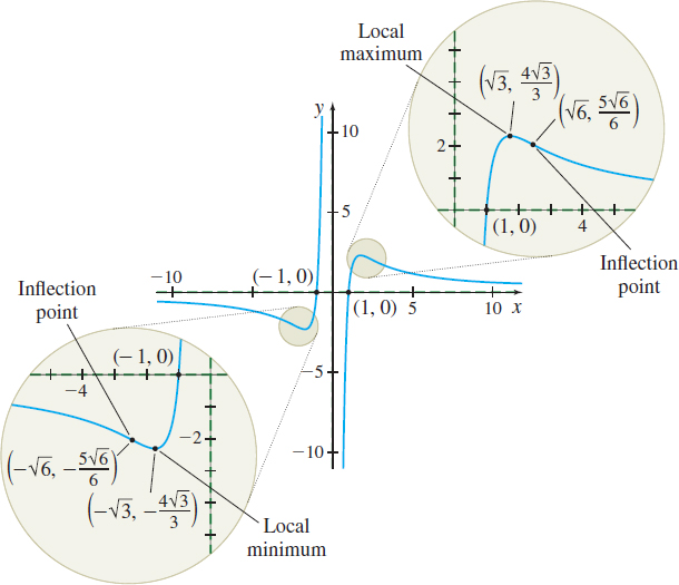
Graph \(f(x)=\dfrac{6x^{2}-6}{x^{3}}\).
Solution We follow the steps for graphing a function.
Step 1 \(f\) is a rational function; the domain of \(f\) is \(\{ x|x\neq 0\} \). The \(x\)-intercepts are \(-1\) and \(1\). There is no \(y\)-intercept. We plot the intercepts \((-1,0)\) and \((1,0) .\)
Step 2 The degree of the numerator is less than the degree of the denominator, so \(f\) has a horizontal asymptote. We find the horizontal asymptotes by finding the limits at infinity. Using L’Hôpital’s Rule, we get \[ \lim\limits_{x\rightarrow \infty }\frac{6x^{2}-6}{x^{3}}=\lim\limits_{x \rightarrow \infty }\dfrac{12x}{3x^{2}}=\lim\limits_{x\rightarrow \infty } \frac{12}{6x}=0 \]
The line \(y=0\) is a horizontal asymptote as \(x\rightarrow -\infty\) and as \(x\rightarrow \infty \).
We identify vertical asymptotes by checking for infinite limits. [\(\lim\limits_{x\rightarrow 0}f(x) \) is the only one to check–do you see why?] \[ \lim\limits_{x\rightarrow 0^{-}}{\frac{6x^{2}-6}{x^{3}}}=\infty \qquad \lim\limits_{x\rightarrow 0^{+}}{\frac{6x^{2}-6}{x^{3}}} =-\infty \]
The line \(x=0\) is a vertical asymptote. We draw the asymptotes on the graph.
310
Step 3 \[ \begin{array}{l} f'(x) &=& \frac{d}{{dx}}\left( {\frac{{6x^2 - 6}}{{x^3 }}} \right) = \frac{{12x(x^3 ) - (6x^2 - 6)(3x^2 )}}{{x^6 }} \\ &=& \frac{{6x^2 (3 - x^2 )}}{{x^6 }} = \frac{{6(3 - x^2 )}}{{x^4 }} \\ f''(x) &=& \frac{d}{{dx}}\left[ {\frac{{6(3 - x^2 )}}{{x^4 }}} \right] = 6 \cdot \frac{{( - 2x)x^4 - (3 - x^2 )(4x^3 )}}{{x^8 }} \\ &=& \frac{{12x^3 (x^2 - 6)}}{{x^8 }} = \frac{{12(x^2 - 6)}}{{x^5 }} \\ \end{array} \]
Critical numbers occur where \(f^\prime (x) =0\) or where \(f^\prime (x)\) does not exist. Since \(f^\prime (x) =0\) when \(x=\pm \sqrt{3}\), there are two critical numbers, \(\sqrt{3}\) and \(-\sqrt{3}\). (The derivative does not exist at \(0\), but, since \(0\) is not in the domain of \(f\), it is not a critical number.)
Step 4 To apply the Increasing/Decreasing Function Test, we use the numbers \(-\sqrt{3},\) \(0,\) and \(\sqrt{3}\) to form four intervals.
| Interval | Sign of f\(^\prime\) | Conclusion |
|---|---|---|
| \(( -\infty ,-\sqrt{3})\) | negative | \(f\) is decreasing on \(( -\infty ,-\sqrt{3})\) |
| \(( -\sqrt{3},0)\) | positive | \(f\) is increasing on \(( - \sqrt{3},0)\) |
| \((0,\sqrt{3})\) | positive | \(f\) is increasing on \(( 0, \sqrt{3})\) |
| \(( \sqrt{3},\infty )\) | negative | \(f\) is decreasing on \(( \sqrt{3},\infty )\) |
Step 5 We use the First Derivative Test. From the table in Step 4, we conclude
- \(f( -\sqrt{3}) =\) \(-\dfrac{4}{\sqrt{3 }}\approx -2.31\) is a local minimum value.
- \(f(\sqrt{3}) =\) \(\dfrac{4}{\sqrt{3}}\approx 2.31\) is a local maximum value
Plot the local extreme points.
Step 6 We use the Test for Concavity. \(f^{\prime \prime} (x) =\dfrac{12( x^{2}-6) }{x^{5}}=0\) when \(x=\pm \sqrt{6}\). Now use the numbers \(-\sqrt{6},\) \(0,\) and \(\sqrt{6}\) to form four intervals.
| Interval | Sign of f\(^{\prime \prime}\) | Conclusion |
|---|---|---|
| \(( -\infty ,-\sqrt{6})\) | negative | \(f\) is concave down on \(( -\infty ,-\sqrt{6})\) |
| \((-\sqrt{6},0)\) | positive | \(f\) is concave up on \(( -\sqrt{6},0)\) |
| \( 0,\sqrt{6}\) | negative | \(f\) is concave down on \(( 0,\sqrt{6})\) |
| \(( \sqrt{6},\infty )\) | positive | \(f\) is concave up on \(( \sqrt{6},\infty )\) |
The concavity of the function \(f\) changes at \(-\sqrt{6},\) \(0,\) and \(\sqrt{6}\). So, theeak points \(\left( -\sqrt{6},-\dfrac{5\sqrt{6}}{6}\right)\) and \(\left( \sqrt{6},\dfrac{5\sqrt{6}}{6}\right)\) are inflection points. Since \(0\) is not in the domain of \(f,\) there is no inflection point at \(0.\) We plot the inflectioneak points.
Step 7 We now use the information about where the function increases/decreases and the concavity to complete the graph. See Figure 47. Notice the apparent symmetry of the graph with respect to the origin. We can verify this symmetry by showing \(f( -x) =-f(x)\) and concluding that \(f\) is an odd function.
311
NOW WORK
Problem 9.
Some functions have a graph with an oblique asymptote. That is, the graph of the function approaches a line \(y=mx+b,\) \(m\neq 0,\) as \(x\) becomes unbounded in either the positive or negative direction.
In general, for a function \(y=f(x)\), the line \(y=mx+b,\) \(m\neq 0, \) is an oblique asymptote of the graph of \(f\), if \[ \lim\limits_{x\rightarrow -\infty }[ f(x) -( mx+b) ] =0\qquad\hbox{or}\qquad\lim\limits_{x \rightarrow \infty }[ f(x) -( mx+b) ] =0 \]
In Chapter 1, we saw that rational functions can have vertical or horizontal asymptotes. Rational functions can also have oblique asymptotes, but cannot have both a horizontal asymptote and an oblique asymptote. Rational functions for which the degree of the numerator is 1 more than the degree of the denominator have an oblique asymptote; rational functions for which the degree of the numerator is less than or equal to the degree of the denominator have a horizontal asymptote.
Using Calculus to Graph a Rational Function
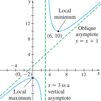
Graph \(f(x) =\dfrac{x^{2}-2x+6}{x-3}\).
Solution
Step 1 \(f\) is a rational function; the domain of \(f\) is \(\{ x|x\neq 3\}\). There are no \(x\)-intercepts, since \( x^{2}-2x+6=0\) has no real solutions. (Its discriminant is negative.) The \(y\) -intercept is \(f( 0) =-2\). Plot the intercept \(( 0,-2).\)
Step 2 We identify any vertical asymptotes by checking for infinite limits (\(3\) is the only number to check). Since \(\lim\limits_{x\rightarrow 3^{-}}\left( \dfrac{x^{2}-2x+6}{x-3}\right) =-\infty \) and \(\lim\limits_{x\rightarrow 3^{+}}\left( \dfrac{x^{2}-2x+6}{x-3 }\right) =\infty \), the line \(x=3\) is a vertical asymptote.
312
The degree of the numerator of \(f\) is 1 more than the degree of the denominator, so \(f\) will have an oblique asymptote. We divide \(x^{2}-2x+6\) by \( x-3\) to find the line \(y=mx+b\). \[ f(x) =\frac{x^{2}-2x+6}{x-3}=x+1+\frac{9}{x-3} \]
Since \( \lim\limits_{x\rightarrow \infty }[ f(x) -( x+1) ] =\lim\limits_{x\rightarrow \infty }\dfrac{9}{x-3}=0,\) then \(y=x+1\) is an oblique asymptote of the graph of \(f\). Draw the asymptotes on the graph.
Step 3\[ \begin{eqnarray*} f^\prime (x) &=&\dfrac{d}{\textit{dx}}\left( \dfrac{x^{2}-2x+6}{x-3}\right) =\dfrac{( 2x-2) (x-3) -( x^{2}-2x+6) ( 1) }{(x-3) ^{2}}\\ &=&\dfrac{ x^{2}-6x}{(x-3)^{2}}=\dfrac{x( x-6) }{(x-3) ^{2}}\\ f^{\prime \prime} (x) &=&\dfrac{d}{\textit{dx}}\left[ \dfrac{x^{2}-6x}{ (x-3) ^{2}}\right] =\dfrac{( 2x-6) (x-3) ^{2}-( x^{2}-6x) [ 2(x-3) ] }{(x-3) ^{4}} \\ &=&(x-3) \dfrac{( 2x^{2}-12x+18) -( 2x^{2}-12x) }{(x-3) ^{4}}=\dfrac{18}{(x-3) ^{3} } \end{eqnarray*} \]
\(f^\prime (x) =0\) at \(x=0\) and at \(x=6\). So, \(0\) and \(6\) are critical numbers. The tangent lines are horizontal at \(0\) and at \(6.\) Since \(3\) is not in the domain of \(f\), \(3\) is not a critical number.
Step 4 To apply the Increasing/Decreasing Function Test, we use the numbers \(0,\) \(3,\) and \(6\) to form four intervals.
| Interval | Sign of f\(^\prime(x)\) | Conclusion |
|---|---|---|
| \((-\infty ,0)\) | positive | \(f\) is increasing on \((-\infty ,0)\) |
| \((0,3)\) | negative | \(f\) is decreasing on \((0,3)\) |
| \(\left( 3,6\right)\) | negative | \(f\) is decreasing on \(\left( 3,6\right)\) |
| \(\left( 6,\infty \right)\) | positive | \(f\) is increasing on \(\left(6,\infty \right) \) |
Step 5 Using the First Derivative Test, we find that \(f( 0) =-2\) is a local maximum value and \(f( 6) =10\) is a local minimum value. Plot the points \(\left( 0,-2\right)\) and \(\left( 6,10\right)\).
Step 6 \(f^{\prime \prime} (x) =\dfrac{18}{(x-3) ^{3}}\). If \(x<3\), \(f^{\prime \prime} (x) <0\), and if \(x>3\) , \(f^{\prime \prime} (x) >0\). From the Test for Concavity, we conclude \(f\) is concave down on the interval \(\left( -\infty ,3\right)\) and \(f\) is concave up on the interval \((3,\infty) \). The concavity changes at \(3\), but \(3\) is not in the domain of \(f\). So, the graph of \(f\) has no inflection point.
Step 7 We use the information to complete the graph of the function. See Figure 48.
NOW WORK
Problem 11.
Using Calculus to Graph a Function
Graph \(\ f(x)=\dfrac{x}{\sqrt{x^{2}+4}}\).
Solution
Step 1 The domain of \(f\) is all real numbers. The only intercept is \((0,0)\). So, we plot the point \((0,0) .\)
Step 2 We check for horizontal asymptotes. Since \[ \begin{eqnarray*} \lim\limits_{x\rightarrow \infty }f(x) =\lim\limits_{x\rightarrow \infty }\dfrac{x}{\sqrt{x^{2}+4}}=\sqrt{ \lim\limits_{x\rightarrow \infty }\dfrac{x^{2}}{x^{2}+4}} \underset{\underset{{\color{#0066A7}{\hbox{L’Hôpital’s Rule}}}} {\color{#0066A7}{{{\left\uparrow{\vphantom{width0pc height9pt depth0pt}}\right.}}}}}{=} \sqrt{\lim\limits_{x\rightarrow \infty }\dfrac{2x}{2x}}=1\\[-12.9pt] \end{eqnarray*} \]
the line \(y=1\) is a horizontal asymptote as \(x\rightarrow \infty .\) Since \(\lim\limits_{x\rightarrow -\infty }f(x) =-1,\) the line \(y=-1\) is also a horizontal asymptote as \(x\rightarrow -\infty .\) We draw the horizontal asymptotes on the graph.
313
Since \(f\) is defined for all real numbers, there are no vertical asymptotes.
Step 3\[ \begin{array}{@{\hspace*{-2.6pc}}rcl} \!\!f^\prime (x) &=&\dfrac{d}{\textit{dx}}\left( \dfrac{x }{\sqrt{x^{2}+4}}\right) =\dfrac{1\cdot \sqrt{x^{2}+4}-x\left[ \dfrac{1}{2} ( x^{2}+4) ^{-1/2}\cdot 2x\right] }{x^{2}+4}\\[5pt] &=&\dfrac{\sqrt{x^{2}+4}-\dfrac{x^{2}}{\sqrt{x^{2}+4}}}{x^{2}+4} =\dfrac{x^{2}+4-x^{2}}{( x^{2}+4) \sqrt{x^{2}+4}}=\dfrac{4}{(x^{2}+4)^{3/2}}\\ f^{\prime \prime} (x) &=& \dfrac{d}{\textit{dx}} \left[ \dfrac{4}{( x^{2}+4) ^{3/2}}\right] =4\left[ -\dfrac{3}{2} ( x^{2}+4) ^{-5/2}\right] \cdot 2x=\dfrac{-12x}{( x^{2}+4) ^{5/2}} \end{array} \]
Since \(f^\prime (x)\) is never \(0\) and \(f^\prime\) exists for all real numbers, there are no critical numbers.
Step 4 Since \(f^\prime (x) >0\) for all \(x\), \(f\) is increasing on \(( -\infty ,\infty)\) .
Step 5 Because there are no critical numbers, there are no local extreme values.
Step 6 We test for concavity. Since \(f^{\prime \prime} (x) >0\) on the interval \((-\infty ,0) \), \(f\) is concave up on \((-\infty ,0)\); and since \(f^{\prime \prime} (x) <0\) on the interval \(( 0,\infty ) \), \(f\) is concave down on \(( 0,\infty ) \). The concavity changes at \(0,\) and \(0\) is in the domain of \(f\), so the point \((0,0)\) is an inflection point of \(f\). Plot the inflection point.
Step 7 Figure 49 shows the graph of \(f\).
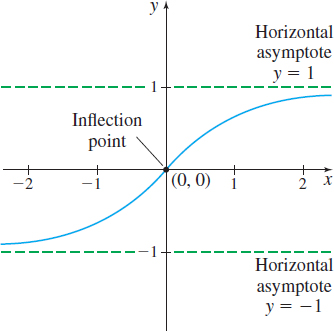
Notice the apparent symmetry of the graph with respect to the origin. We can verify this by showing \(f( -x) =-f(x) ,\) that is, by showing \(f\) is an odd function.
NOW WORK
Problem 25.
Using Calculus to Graph a Function
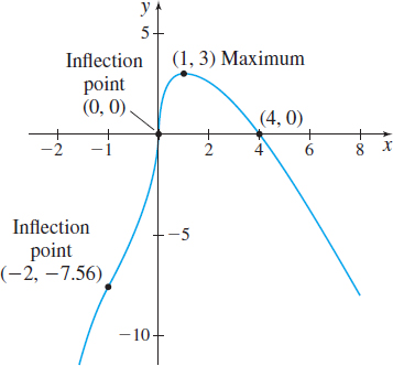
Graph \(f(x)=4x^{1/3}-x^{4/3}\).
Solution
Step 1 The domain of \(f\) is all real numbers. Since \(f(0) = 0\), the \(y\)-intercept is \(0\). Now \(f(x) = 0\) when \(4x^{1/3}-x^{4/3}=x^{1/3}\left( 4-x\right) =0\) or when \(x=0\) or \(x=4.\) So, the \(x\)-intercepts are \(0\) and \(4\). Plot the intercepts \((0,0)\) and \(\left( 4,0\right).\)
Step 2 Since \(\lim\limits_{x\rightarrow \infty }f(x) =\lim\limits_{x\rightarrow \infty }[ x^{1/3}(4-x)] =-\infty\), there is no horizontal asymptote. Since the domain of \(f\) is all real numbers, there is no vertical asymptote.
Step 3 \[ \begin{eqnarray*} f^\prime (x) &=&\dfrac{d}{\textit{dx}}( 4x^{1/3}-x^{4/3}) =\dfrac{4}{3}x^{-2/3}-\dfrac{4}{3}x^{1/3} = \dfrac{4}{3}\!\left( \dfrac{1}{x^{2/3}}-x^{1/3}\right)\\[5pt] &=&\dfrac{4}{3}\!\left( \dfrac{1-x}{ x^{2/3}}\right) \\[5pt] f^{\prime \prime} (x) &=&\dfrac{d}{\textit{dx}}\!\left( \dfrac{4}{ 3}x^{-2/3}-\dfrac{4}{3}x^{1/3}\right) =-\dfrac{8}{9}x^{-5/3}-\dfrac{4}{9} x^{-2/3}=-\dfrac{4}{9}\!\left( \dfrac{2}{x^{5/3}}+\dfrac{1}{x^{2/3}}\right)\\[5pt] &=&-\dfrac{4}{9}\cdot \dfrac{2+x}{x^{5/3}} \end{eqnarray*} \]
Since \(f^\prime (x) =\dfrac{4}{3}\!\left( \dfrac{1-x}{ x^{2/3}}\right) =0\) when \(x=1\) and \(f^\prime (x)\) does not exist at \(x = 0,\) the critical numbers are \(0\) and \(1\). At the point \((1,3)\), the tangent line to the graph is horizontal; at the point \((0,0)\), the tangent line is vertical. Plot these points.
314
Step 4 To apply the Increasing/Decreasing Function Test, we use the critical numbers \(0\) and \(1\) to form three intervals.
| Interval | Sign of f\(^\prime\) | Conclusion |
|---|---|---|
| \((-\infty ,0)\) | positive | \(f\) is increasing on \((-\infty ,0)\) |
| (0,1) | positive | \(f\) is increasing on \((0,1)\) |
| \((1,\infty)\) | negative | \(f\) is decreasing on \((1,\infty )\) |
Step 5 By the First Derivative Test, \(f( 1) =3\) is a local maximum value and \(f( 0) =0\) is not a local extreme value.
Step 6 We now test for concavity by using the numbers \(-2\) and \( 0 \) to form three intervals.
| Interval | Sign of f\(^{\prime \prime}\) | Conclusion |
|---|---|---|
| \(( -\infty ,-2)\) | negative | \(f\) is concave down on the interval \(( -\infty ,-2)\) |
| (–2,0) | positive | \(f\) is concave up on the interval \(( -2,0)\) |
| \(( 0,\infty )\) | negative | \(f\) is concave down on the interval \(( 0,\infty )\) |
The concavity changes at \(-2\) and at \(0.\) Since \[ f( -2) =4( -2) ^{1/3}- ( -2) ^{4/3}= 4\sqrt[3]{-2}-\sqrt[3]{16}\approx -7.56, \]
the inflection points are \(( -2,-7.56)\) and \((0,0)\) . Plot the inflection points.
Step 7 The graph of \(f\) is given in Figure 50.
NOW WORK
Problem 19.
Using Calculus to Graph a Trigonometric Function
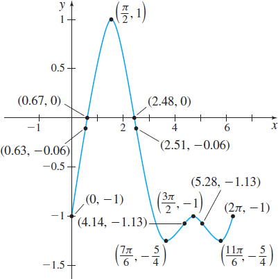
Graph \(f(x)=\sin x-\cos ^{2}x,\) \(0\leq x\leq 2\pi\) .
Solution
Step 1 The domain of \(f\) is \(\{ x|0\leq x\leq 2\pi \} \). Since \(f( 0) =\sin 0-\cos ^{2}0=-1\), the \(y\)-intercept is \(-1\). The \(x\)-intercepts satisfy the equation \[ \sin x-\cos ^{2}x=\sin x-( 1-\!\sin ^{2}x) =\sin ^{2}x+\sin x-1=0 \]
This trigonometric equation is quadratic in form, so we use the quadratic formula. \[ \sin x=\dfrac{-1\pm \sqrt{1-4( 1) (-1) }}{2}=\dfrac{ -1\pm \sqrt{5}}{2} \]
NEED TO REVIEW?
Trigonometric equations are discussed in Section P.7, pp. 61-63.
Since \(\dfrac{-1-\sqrt{5}}{2}<-1\) and \(-1\leq \sin x\leq 1\), the \(x\) -intercepts occur at \(x=\sin ^{-1}\left( \dfrac{-1+\sqrt{5}}{2}\right) \approx 0.67\) and at \(x=\pi -\sin ^{-1}\left( \dfrac{-1+\sqrt{5}}{2}\right) \approx 2.48.\) Plot the intercepts.
Step 2 The function \(f\) has no asymptotes.
Step 3 \[ \begin{array}{@{}rcl} f' (x)&=&\dfrac{d}{\textit{dx}}( \sin x-\cos ^{2} x) =\cos x+2\, \cos\, x\, \sin x=\cos x(1+2\sin x)\\ f'' (x)& =&\dfrac{d}{\textit{dx}}[ {\cos x(1+2\sin x)}] =2\, \cos ^{2}x-\!\sin x(1+2\sin x)\\ &=&2\cos ^{2}x-\!\sin x-2\sin ^{2}x=-4\sin ^{2}x-\!\sin x+2 \end{array} \]
The critical numbers occur where \(f^\prime (x) =0\). That is, where \[ \cos x=0 \qquad\hbox{or}\qquad 1+2\sin x=0 \]
315
In the interval \([0,2\pi ] \): \(\cos x=0\) if \(x=\dfrac{\pi }{2}\) or if \(x=\dfrac{3\pi }{2}\); and \(1+2\sin x=0\) when \(\sin x=-\dfrac{1}{2}\), that is, when \(x=\dfrac{7\pi }{6}\) or \(x=\dfrac{11\pi }{6}\). So, the critical numbers are \(\dfrac{\pi }{2}\), \(\dfrac{7\pi }{6}\), \(\dfrac{3\pi }{2}\), and \(\dfrac{11\pi }{6}\). At each of these numbers, the tangent lines are horizontal.
Step 4 To apply the Increasing/Decreasing Function Test, we use the numbers \(0,\) \(\dfrac{\pi }{2}\), \(\dfrac{7\pi }{6}\), \(\dfrac{3\pi }{2}\), \( \dfrac{11\pi }{6},\) and \(2\pi\) to form five intervals.
| Interval | Sign of fs\(^\prime\) | Conclusion |
|---|---|---|
| \(\left( 0,\dfrac{\pi }{2}\right)\) | positive | \(f\) is increasing on \(\left( 0,\dfrac{\pi }{2}\right)\) |
| \(\left( \dfrac{\pi }{2},\dfrac{7\pi }{6}\right)\) | negative | \(f\) is decreasing on \(\left( \dfrac{\pi }{2},\dfrac{7\pi}{6}\right)\) |
| \(\left(\dfrac{7\pi}{6},\dfrac{3\pi}{2}\right)\) | positive | \(f\) is increasing on \(\left( \dfrac{7\pi }{6},\dfrac{3\pi}{2}\right)\) |
| \(\left( \dfrac{3\pi }{2},\dfrac{11\pi }{6}\right)\) | negative | \(f\) is decreasing on \(\left( \dfrac{3\pi }{2},\dfrac{11\pi }{6}\right)\) |
| \(\left( \dfrac{11\pi }{6},2\pi \right)\) | positive | \(f\) is increasing on \(\left( \dfrac{11\pi }{6},2\pi \right)\) |
Step 5 By the First Derivative Test, \(f\left( \dfrac{\pi }{2} \right) =1\) and \(f\left( \dfrac{3\pi }{2}\right) =-1\) are local maximum values, and \(f\left(\dfrac{7\pi}{6}\right) =-\dfrac{5}{4}\) and \(f\left(\dfrac{11\pi}{6}\right) =-\dfrac{5}{4}\) are local minimum values. Plot these points.
Step 6 We apply the Test for Concavity. To solve \(f^{\prime \prime} (x) >0\) and \(f^{\prime \prime} (x) <0\), we first solve the equation \(f^{\prime \prime} (x) =-4\sin ^{2}x-\!\sin x+2=0,\) or equivalently, \[ \begin{eqnarray*} 4\sin ^{2}x+\sin x-2 &=&0 \qquad 0\leq x\leq 2\pi \\[3pt] \sin x &=&\dfrac{-1\pm \sqrt{1+32}}{8} \\[3pt] \sin x &\approx &0.593\qquad \hbox{or}\qquad \sin x\approx -0.843 \\ x &\approx &0.63 \qquad x\approx 2.51 \qquad x\approx 4.14 \qquad x\approx 5.28 \end{eqnarray*} \]
We use these numbers to form five subintervals of \([0,2\pi ]\).
| Interval | Sign of f\(^{\prime \prime}\) | Conclusion |
|---|---|---|
| \((0,0.63)\) | positive | \(f\) is concave up on the interval \(( 0,0.63)\) |
| \(( 0.63,2.51)\) | negative | \(f\) is concave down on the interval \(( 0.63,2.51)\) |
| \(( 2.51,4.14)\) | positive | \(f\) is concave up on the interval \(( 2.51,4.14)\) |
| \(( 4.14,5.28)\) | negative | \(f\) is concave down on the interval \(( 4.14,5.28)\) |
| \(( 5.28,2\pi )\) | positive | \(f\) is concave up on the interval \(( 5.28,2\pi )\) |
The inflection points are \(( 0.63,-0.06) \), \((2.51,-0.06) \), \(( 4.14,-1.13) \), and \(( 5.28,-1.13) .\) Plot the inflection points.
NOTE
The function \(f\) in Example 6 is periodic with period \(2\pi\). To graph this function over its unrestricted domain, the set of real numbers, repeat the graph in Figure 51 over intervals of length \(2\pi\).
Step 7 The graph of \(f\) is given in Figure 51.
NOW WORK
Problem 33.
316
Using Calculus to Graph a Function
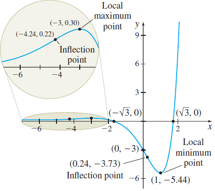
Graph \(f(x)=e^{x}( x^{2}-3) \).
Solution
Step 1 The domain of \(f\) is all real numbers. Since \(f( 0) =-3\), the \(y\)-intercept is \(-3\). The \(x\) -intercepts occur where \[ \begin{eqnarray*} f(x) &=&e^{x}( x^{2}-3) =0 \\[3pt] x &=&\sqrt{3}\qquad\hbox{or}\qquad x=-\sqrt{3} \end{eqnarray*} \]
Plot the intercepts.
Step 2 Since the domain of \(f\) is all real numbers, there are no vertical asymptotes. To determine if there is a horizontal asymptote, we find the limits at infinity. \[ \lim\limits_{x\rightarrow -\infty }f(x) =\lim\limits_{x\rightarrow -\infty } [ e^{x} ( x^{2}-3 ) ] \]
Since \(e^{x} ( x^{2}-3 )\) is an indeterminate form at \(-\infty\) of the type \(0\cdot \infty \), we write \(e^{x} ( x^{2}-3 ) =\dfrac{x^{2}-3}{e^{-x}}\) and use L’Hôpital’s Rule.
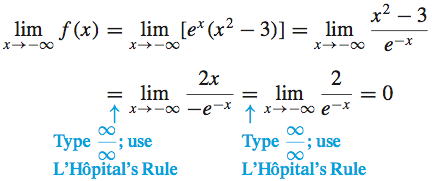
The line \(y=0\) is a horizontal asymptote as \(x\rightarrow -\infty\).
Since \( \lim\limits_{x\rightarrow \infty }[ e^{x}( x^{2}-3) ] =\infty ,\) there is no horizontal asymptote as \(x\rightarrow \infty .\) Draw the asymptote on the graph.
Step 3 \[ \begin{array}{@{}rcl} f^\prime (x) &=&\dfrac{d}{\textit{dx}}[e^{x}( x^{2}-3) ] =e^{x}(2x) +e^{x}(x^{2}-3) =e^{x}( x^{2}+2x-3)\\[8pt] &=&e^{x}( x+3) ( x-1)\\[11pt] f^{\prime \prime} (x) &=&\dfrac{d}{\textit{dx}}[e^{x}( x^{2}+2x-3) ] =e^{x}( 2x+2) +e^{x}(x^{2}+2x-3)\\[8pt] &=&e^{x}( x^{2}+4x-1) \end{array} \]
Solving \(f^\prime (x) =0,\) we find that the critical numbers are \(-3\) and \(1\).
Step 4 To apply the Increasing/Decreasing Function Test, we use the critical numbers \(-3\) and \(1\) to form three intervals.
| Interval | Sign of f\(^\prime\) | Conclusion |
|---|---|---|
| \(( -\infty ,-3)\) | positive | \(f\) is increasing on the interval \(( -\infty ,-3)\) |
| \((-3,1)\) | negative | \(f\) is decreasing on the interval \(( -3,1)\) |
| \((1,\infty )\) | positive | \(f\) is increasing on the interval \( (1,\infty )\) |
Step 5 We use the First Derivative Test to identify the local extrema. From the table in Step 4, there is a local maximum at \(-3\) and a local minimum at \(1.\) Then \(f(-3) =6e^{-3}\approx 0.30\) is a local maximum value and \(f(1) =-2e\approx -5.44\) is a local minimum value. Plot the local extrema.
317
Step 6 To determine the concavity of \(f,\) first we solve \( f^{\prime \prime} (x) =0\). We find \(x=-2\pm \sqrt{5}\). Now we use the numbers \(-2-\sqrt{5}\approx -4.24\) and \(-2+\sqrt{5}\approx 0.24\) to form three intervals and apply the Test for Concavity.
| Interval | Sign of \({f''}\) | Conclusion |
|---|---|---|
| \(( -\infty ,-2-\sqrt{5})\) | positive | \(f\) is concave up on the interval \((-\infty ,-2 - \sqrt{5})\) |
| \((-2-\sqrt{5},-2+\sqrt{5})\) | negative | \(f\) is concave down on the interval \(( -2 -\sqrt{5}, -2+\sqrt{5})\) |
| \((-2+\sqrt{5},\infty)\) | positive | \(f\) is concave up on the interval \(( -2+\sqrt{5},\infty )\) |
The inflection points are \(( -4.24,0.22) \) and \(( 0.24,-3.73) .\) Plot the inflection points.
Step 7 The graph of \(f\) is given in Figure 52.
NOW WORK
Problem 39.