4.4 Local Extrema and Concavity
OBJECTIVES
When you finish this section, you should be able to:
- Use the First Derivative Test to find local extrema (p. 284)
- Use the First Derivative Test with rectilinear motion (p. 286)
- Determine the concavity of a function (p. 287)
- Find inflection points (p. 290)
- Use the Second Derivative Test to find local extrema (p. 291)
So far we know that if a function \(f\) defined on a closed interval has a local maximum or a local minimum at a number \(c\) in the open interval, then \(c\) is a critical number. We are now ready to see how the derivative is used to determine whether a function \(f\) has a local maximum, a local minimum, or neither at a critical number.
1 Use the First Derivative Test to Find Local Extrema
All local extreme values of a function \(f\) occur at critical numbers. While the value of \(f\) at each critical number is a candidate for being a local extreme value for \(f\), not every critical number gives rise to a local extreme value.
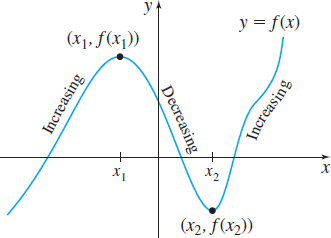
How do we distinguish critical numbers that give rise to local extreme values from those that do not? And then how do we determine if a local extreme value is a local maximum value or a local minimum value? Figure 30 provides a clue. If you look from left to right along the graph of \(f\), you see that the graph of \(f\) is increasing to the left of \(x_{1}\), where a local maximum occurs, and is decreasing to its right. The function \(f\) is decreasing to the left of \(x_{2}\), where a local minimum occurs, and is increasing to its right. So, knowing where a function \(f\) increases and decreases enables us to find local maximum values and local minimum values.
The next theorem is usually referred to as the First Derivative Test, since it relies on information obtained from the first derivative of a function.
IN WORDS
If \(c\) is a critical number of \({f}\) and if \({f}\) is increasing to the left of \({c}\) and decreasing to the right of \({c},\) then \({f}({c})\) is a local maximum value. If \({f}\) is decreasing to the left of \({c}\) and increasing to the right of \({c}\), then \({f}({c})\) is a local minimum value.
THEOREM First Derivative Test
Let \(f\) be a function that is continuous on an interval \(I\). Suppose that \(c\) is a critical number of \(f\) and \((a,b)\) is an open interval in \(I\) containing \(c\):
- If \(f^\prime (x)>0\) for \(a<x<c\) and \(f^\prime (x) <0\) for \(c<x<b\), then \(f(c)\) is a local maximum value.
- If \(f^\prime (x)<0\) for \(a<x<c\) and \(f^\prime (x) >0\) for \(c<x<b\), then \(f(c)\) is a local minimum value.
- If \(f^\prime (x)\) has the same sign on both sides of \(c\), then \(f(c)\) is neither a local maximum value nor a local minimum value.
285
Partial Proof
If \(f^\prime (x)>0\) on the interval \((a,c)\), then \(f\) is increasing on \((a,c)\). Also, if \(f^\prime (x)<0\) on the interval \((c,b)\), then \(f\) is decreasing on \((c,b)\). So, for all \(x\) in \(( a,b)\), \(f(x)\leq f(c)\). That is, \(f(c)\) is a local maximum value. See Figure 31(a).
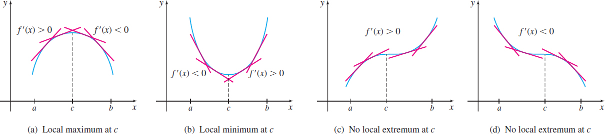
The proofs of the second and third bullets are left as exercises (see Problems 130 and 131). See Figure 31(b) for an illustration of a local minimum value. In Figures 31(c) and 31(d), \(f^\prime\) has the same sign on both sides of \(c\), so \(f\) has neither a local maximum nor a local minimum at \(c\).
Using the First Derivative Test to Find Local Extrema
Find the local extrema of \(f(x)=x^{4}-4x^{3}\).
Solution Since \(f\) is a polynomial function, \(f\) is continuous and differentiable at every real number. We begin by finding the critical numbers of \(f\). \[ f^\prime (x) =4x^{3}-12x^{2}=4x^{2}({x-3}) \]
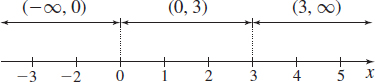
The critical numbers are \(0\) and \(3\). We use the critical numbers \(0\) and \(3\) to form three intervals, as shown in Figure 32. Then we determine where \(f\) is increasing and where it is decreasing by determining the sign of \(f^\prime (x)\) in each interval. See Table 3.
| Interval | Sign of \({x^{2}}\) | Sign of \({x-3}\) | Sign of \({f^\prime (x) =4x^{2}(x-3)}\) | Conclusion |
|---|---|---|---|---|
| \((-\infty ,0)\) | Positive \((+)\) | Negative \((-)\) | Negative \((-)\) | \(f\) is decreasing |
| \((0,3)\) | Positive \((+)\) | Negative \((-)\) | Negative \((-)\) | \(f\) is decreasing |
| \((3,\infty)\) | Positive \((+)\) | Positive \((+)\) | Positive \((+)\) | \(f\) is increasing |
Using the First Derivative Test, \(f\) has neither a local maximum nor a local minimum at \(0\), and \(f\) has a local minimum at \(3\). The local minimum value is \(f(3) =-27\).
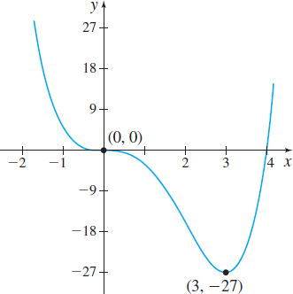
The graph of \(f\) is shown in Figure 33. Notice that the tangent lines to the graph of \(f\) are horizontal at the points \((0,0)\) and \((3,-27)\).
NOW WORK
Problem 13.
Using the First Derivative Test to Find Local Extrema
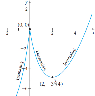
Find the local extrema of \(f(x)=x^{2/3}({x-5})\).
Solution The domain of \(f\) is all real numbers and \(f\) is continuous on its domain. \[ \begin{eqnarray*} &&\hspace{1pc} {f^\prime }(x) = x^{2/3}+\left( {\frac{2}{3}}\right) x^{-1/3}({x-5})=\frac{3x+2({x-5})}{3x^{1/3}}=\frac{5}{3}\!\left( {\frac{x-2}{x^{1/3}}}\right)\\[-10.5pt] && \color{#0066A7}{\underset{\hbox{Use the Product Rule.}}{\uparrow}} \end{eqnarray*} \]
Since \(f^\prime (2) =0\) and \(f^\prime (0)\) does not exist, the critical numbers are \(0\) and \(2\). The graph of \(f\) will have a horizontal tangent line at the point \((2,-3\sqrt[\kern-1pt3\kern1pt]{4})\) and a vertical tangent line at the point \((0,0)\).
286
Table 4 shows the intervals on which \(f\) is increasing and decreasing.
| Interval | Sign of \({x-2}\) | Sign of \({x^{1/3}}\) | Sign of \({f^\prime (x) =\dfrac{5}{3}\left( {\dfrac{x-2}{x^{1/3}}}\right) }\) | Conclusion |
|---|---|---|---|---|
| \((-\infty ,0)\) | Negative \((-)\) | Negative \((-)\) | Positive \((+)\) | \(f\) is increasing |
| \((0,2)\) | Negative \((-)\) | Positive \((+)\) | Negative \((-)\) | \(f\) is decreasing |
| \((2,\infty)\) | Positive \((+)\) | Positive \((+)\) | Positive \((+)\) | \(f\) is increasing |
By the First Derivative Test, \(f\) has a local maximum at \(0\) and a local minimum at \(2\); \(f( 0) =0\) is a local maximum value and \(f(2) =-3\sqrt[3]{4}\) is a local minimum value.
The graph of \(f\) is shown in Figure 34. Notice the vertical tangent line at the point \((0,0)\) and the horizontal tangent line at the point \((2,-3\sqrt[3]{4})\).
NOW WORK
Problem 21.
2 Use the First Derivative Test with Rectilinear Motion
Increasing and decreasing functions can be used to investigate the motion of an object in rectilinear motion. Suppose the distance \(s\) of an object from the origin at time \(t\) is given by the function \(s=f(t)\). We assume the motion is along a horizontal line with the positive direction to the right. The velocity \(v\) of the object is \(v =\dfrac{\textit{ds}}{\textit{dt}}\).
- If \(v =\dfrac{\textit{ds}}{\textit{dt}}\,{>}\,0\), the distance \(s\) from the origin is increasing with time \(t\), and the object moves to the right.
- If \(v =\dfrac{\textit{ds}}{\textit{dt}}\,{<}\,0\), the distance \(s\) from the origin is decreasing with time \(t\), and the object moves to the left.
This information, along with the First Derivative Test, can be used to find the local extreme values of \(s=f(t)\) and to determine at what times \(t\) the direction of the motion of the object changes.
Similarly, if the acceleration of the object, \(a=\dfrac{dv}{\textit{dt}}>0\), then the velocity of the object is increasing, and if \(a=\dfrac{dv}{\textit{dt}}<0\), then the velocity is decreasing. Again, this information, along with the First Derivative Test, is used to find the local extreme values of the velocity.
Using the First Derivative Test with Rectilinear Motion
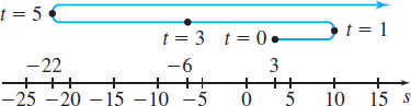
Suppose the distance \(s\) of an object from the origin at time \(t\geq 0,\) in seconds, is given by \[ s=t^{3}-9t^{2}+15t+3 \]
- Determine the time intervals during which the object is moving to the right and to the left.
- When does the object reverse direction?
- When is the velocity of the object increasing and when is it decreasing?
- Draw a figure that illustrates the motion of the object.
- Draw a figure that illustrates the velocity of the object.
287
Solution (a) To investigate the motion, we find the velocity \(v\). \[ v =\frac{\textit{ds}}{\textit{dt}}=3t^{2}-18t+15=3(t^{2}-6t+5)=3(t-1)(t-5) \]
The critical numbers are \(1\) and \(5\). We use Table 5 to describe the motion of the object.
| Time Interval | Sign of \({t-1}\) | Sign of \({t-5}\) | Velocity, \({v}\) | Motion of the Object |
|---|---|---|---|---|
| \((0,1)\) | Negative \((-)\) | Negative \((-)\) | Positive \((+)\) | To the right |
| \((1,5)\) | Positive \((+)\) | Negative \((-)\) | Negative \((-)\) | To the left |
| \((5,\infty )\) | Positive \((+)\) | Positive \((+)\) | Positive \((+)\) | To the right |
The object moves to the right for the first second and again after \(5 \,{\rm seconds}\). The object moves to the left on the interval \((1,5)\).
(b) The object reverses direction at \(t=1\) and \(t=5\).
(c) To determine when the velocity increases or decreases, we find the acceleration. \[ a=\frac{dv }{dt}=6t-18=6(t-3) \]
Since \(a<0\) on the interval \((0,3)\), the velocity \(v\) decreases for the first \(3 \,{\rm seconds}\). On the interval \((3,\infty), a>0\), so the velocity \(v\) increases from \(3 \,{\rm seconds}\) onward.
(d) Figure 35 illustrates the motion of the object.
(e) Figure 36 illustrates the velocity of the object.
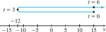
An interesting phenomenon occurs during the first three seconds. The velocity of the object is decreasing on the interval \((0,3)\), as shown Figure 36.
Now, we investigate the speed, namely, \(\vert v(t)\vert =3\vert t^{2}-6t+5\vert =3\vert (t-1) (t-5) \vert\) on the interval \((0,3)\):
- If \(0<t<1\), \(\vert v(t) \vert =3(t^{2}-6t+5)\) and \(\dfrac{d\vert v\vert }{dt}=6(t-3) < 0\), so the speed is decreasing.
- If \(1<t<3\), \(\vert v(t) \vert =-3(t^{2}-6t+5)\) and \(\dfrac{d\vert v\vert }{dt}=-6(t-3) > 0\), so the speed is increasing.
That is, the velocity of the object is decreasing from \(t=0\) to \(t=3\), but its speed is decreasing from \(t=0\) to \(t=1\) and is increasing from \(t=1\) to \(t=3\).
NOW WORK
Problem 35.
3 Determine the Concavity of a Function
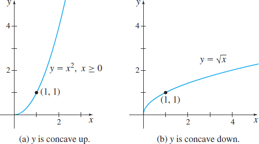
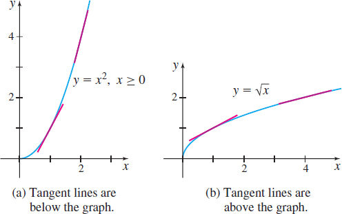
Figure 37 shows the graphs of two familiar functions: \(y=x^{2}\), \(x\ge 0\), and \(y= \sqrt{x}\). Each graph starts at the origin, passes through the point \((1,1)\), and is increasing. But there is a noticeable difference in their shapes. The graph of \(y=x^{2}\) bends upward, it is concave up; the graph of \(y= \sqrt{x}\) bends downward, it is concave down.
288
Suppose we draw tangent lines to the graphs of \(y=x^{2}\) and \(y= \sqrt{x}\), as shown in Figure 38. Notice that the graph of \(y=x^{2}\) lies above all its tangent lines, and moving from left to right, the slopes of the tangent lines are increasing. That is, the derivative \(y^\prime =\dfrac{d}{\textit{dx}}x^{2}\) is an increasing function.
On the other hand, the graph of \(y= \sqrt{x}\) lies below all its tangent lines, and moving from left to right, the slopes of the tangent lines are decreasing. That is, the derivative \(y^\prime =\dfrac{d}{\textit{dx}} \sqrt{x}\) is a decreasing function. This discussion leads to the following definition.
spanDEFINITIONspan Concave Up; Concave Down.
Let \(f\) be a function that is continuous on a closed interval \([a,b]\) and differentiable on the open interval \((a,b)\).
- \(f\) is concave up on \(( a,b)\) if the graph of \(f\) lies above each of its tangent lines throughout \((a,b)\).
- \(f\) is concave down on \(( a,b)\) if the graph of \(f\) lies below each of its tangent lines throughout \((a,b)\).
We can formulate a test to determine where a function \(f\) is concave up or concave down, provided \(f^{\prime \prime}\) exists. Since \(f^{\prime \prime}\) equals the rate of change of \(f^\prime\), it follows that if \(f^{\prime \prime} (x) >0\) on an open interval, then \(f^\prime\) is increasing on that interval, and if \(f^{\prime \prime} (x) <0\) on an open interval, then \(f^\prime\) is decreasing on that interval. As we observed in Figure 38, when \(f^\prime\) is increasing, the graph is concave up, and when \(f^\prime\) is decreasing, the graph is concave down. These observations lead to the test for concavity.
THEOREM Test for Concavity
Let \(f\) be a function that is continuous on a closed interval \([a,b]\). Suppose \(f^\prime\) and \(f^{\prime \prime}\) exist on the open interval \((a,b)\).
- If \(f^{\prime \prime} (x)>0\) on the interval \((a,b)\), then \(f\) is concave up on \(( a,b)\).
- If \(f^{\prime \prime} (x)<0\) on the interval \((a,b)\), then \(f\) is concave down on \(( a,b)\).
Proof
Suppose \(f^{\prime \prime} (x) >0\) on the interval \(( a,b)\), and \(c\) is any fixed number in \((a,b)\). An equation of the tangent line to \(f\) at the point \((c,f(c))\) is \[ y=f(c)+f^\prime (c)(x-c) \]
We need to show that the graph of \(f\) lies above each of its tangent lines for all \(x\) in \(( a,b) .\) That is, we need to show that \[ f(x)\geq f(c)+f^\prime (c) (x-c)\qquad \hbox{ for all }x\hbox{ in }( a,b) \]
If \(x=c\), then \(f(x) = f(c)\) and we are finished.
If \(x\neq c\), then by applying the Mean Value Theorem to the function \(f\), there is a number \(x_{1}\) between \(c\) and \(x\), for which \[ f^\prime (x_{1})=\frac{f(x)-f(c)}{x-c} \]
Now we solve for \(f(x)\): \[\begin{equation*} f(x) =f( c) +f^\prime (x_{1}) (x-c) \tag{1} \end{equation*} \]
There are two possibilities: Either \(c < x_{1} < x\) or \(x < x_{1} < c\).
Suppose \(c<x_{1}<x\). Since \(f^{\prime \prime} (x) >0\) on the interval \((a,b)\), it follows that \(f^\prime\) is increasing on \((a,b)\). For \(x_{1}>c\), this means that \({f^\prime } (x_{1})>{f^\prime } (c)\). As a result, from (1), we have \[ f(x)>f(c)+f^\prime (c)(x-c) \]
289
That is, the graph of \(f\) lies above each of its tangent lines to the right of \(c\) in \((a,b)\).
Similarly, if \(x<x_{1}<c\), then \(f(x) >f( c)+f^\prime ( c) (x-c)\).
In all cases, \(f(x) \geq f(c) + f^\prime (c) (x-c)\) so \(f\) is concave up on \(( a,b)\).
The proof that if \(f^{\prime \prime} (x) <0,\) then \(f\) is concave down is left as an exercise. See Problem 132.
Determining the Concavity of \(f(x)=e^x\)
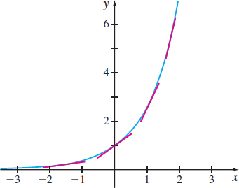
Show that \(f(x)=e^{x}\) is concave up on its domain.
Solution The domain of \(f(x) =e^{x}\) is all real numbers. The first and second derivatives of \(f\) are \[ f^\prime (x)=e^{x}\qquad f^{\prime \prime} (x)=e^{x} \]
Since \(f^{\prime \prime} (x) >0\) for all real numbers, by the Test for Concavity, \(f\) is concave up on its domain.
Figure 39 shows the graph of \(f(x) =e^{x}\) and a selection of tangent lines to the graph. Notice that for any \(x,\) the graph of \(f\) lies above its tangent lines.
NOW WORK
Problem 45(a).

Finding Local Extrema and Determining Concavity
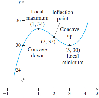
- Find any local extrema of the function \(f(x)=x^{3}-6x^{2}+9x+30\).
- Determine where \(f(x)=x^{3}-6x^{2}+9x+30\) is concave up and where it is concave down.
Solution (a) The first derivative of \(f\) is \[ f^\prime (x)=3x^{2}-12x+9=3( x-1) (x-3) \]
So, \(1\) and \(3\) are critical numbers of \(f.\) Now,
- \(f^\prime (x)=3( x-1) (x-3) >0\) if \(x<1\) or \(x>3\).
- \(f^\prime (x) <0\) if \(1<x<3\).
So \(f\) is increasing on \(( -\infty ,1)\) and on \((3,\infty)\); \(f\) is decreasing on \((1,3)\).
At \(1,\) \(f\) has a local maximum, and at \(3\), \(f\) has a local minimum. The local maximum value is \(f( 1) = 34\); the local minimum value is \(f(3) =30\).
(b) To determine concavity, we use the second derivative: \[ f^{\prime \prime} (x)=6x-12= 6(x-2) \]
Now, we solve the inequalities \(f^{\prime \prime} (x) <0\) and \(f^{\prime \prime} (x) >0\) and use the Test for Concavity.
- \(f^{\prime \prime} (x) < 0 \qquad \hbox{ if }x<2,\qquad \hbox{ so }f \hbox{ is concave down on }( -\infty ,2)\)
- \(f^{\prime \prime} (x) > 0 \qquad \hbox{ if }x>2,\qquad \hbox{ so }f \hbox{ is concave up on }(2,\infty )\)
Figure 40 shows the graph of \(f\). The point \(( 2,32)\) where the concavity of \(f\) changes is of special importance and is called an inflection point.
spanDEFINITIONspan Inflection Point
Suppose \(f\) is a function that is differentiable on an open interval \((a,b)\) containing \(c\). If the concavity of \(f\) changes at the point \((c, f(c))\), then \((c, f(c))\) is an inflection point of \(f\).
4 Find Inflection Points
290
If \((c,\;f(c))\) is an inflection point of \(f\), then on one side of \(c\) the slopes of the tangent lines are increasing (or decreasing), and on the other side of \(c\) the slopes of the tangent lines are decreasing (or increasing). This means the derivative \(f^\prime\) must have a local maximum or a local minimum at \(c\). In either case, it follows that \(f^{\prime \prime} ( c) =0\) or \(f^{\prime \prime} (c)\) does not exist.
THEOREM A Condition for an Inflection Point
Let \(f\) denote a function that is differentiable on an open interval \((a,\;b)\) containing \(c\). If \((c,\;f(c))\) is an inflection point of \(f\), then either \(f^{\prime \prime} (c) =0\) or \(f^{\prime \prime}\) does not exist at \(c\).
Notice the wording in the theorem. If you know that \((c,\;f( c))\) is an inflection point of \(f\), then the second derivative of \(f\) at \(c\) is \(0\) or does not exist. The converse is not necessarily true. In other words, a number at which \(f^{\prime \prime}(x)=0\) or at which \(f^{\prime \prime}\) does not exist will not always identify an inflection point.
Steps for Finding the Inflection Points of a Function \(f\)
Step 1 Find all numbers in the domain of \(f\) at which \(f^{\prime \prime} (x)=0\) or at which \(f^{\prime \prime}\) does not exist.
Step 2 Use the Test for Concavity to determine the concavity of \(f\) on both sides of each of these numbers.
Step 3 If the concavity changes, there is an inflection point; otherwise, no inflection point exists.
Finding Inflection Points
Find the inflection points of \(f(x)=x^{5/3}\).
Solution We follow the steps for finding an inflection point.
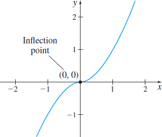
Step 1 The domain of \(f\) is all real numbers. The first and second derivatives of \(f\) are \[ {f^\prime (x)=\frac{5}{3}x^{2/3}}\qquad f^{\prime \prime} (x)=\frac{10}{9}x^{-1/3}=\frac{10}{9x^{1/3}} \]
The second derivative of \(f\) does not exist when \(x =0\). So, \((0,0)\) is a possible inflection point.
Step 2 Now use the Test for Concavity.
- \(\hbox{If }x<0\quad \text{then}\quad\) \(f^{\prime\prime} (x)<0\) \(\hbox{ so }f\hbox{ is concave down on}\;(-\infty ,0).\)
- \(\hbox{If }x>0\quad \text{then}\quad\) \(f^{\prime\prime} (x)>0\) \(\hbox{ so }f\hbox{ is concave up on }\;(0,\infty ).\)
Step 3 Since the concavity of \(f\) changes at \(0\), we conclude that \((0,0)\) is an inflection point of \(f.\)
Figure 41 shows the graph of \(f\).
NOW WORK
Problems 45(b) and 51.
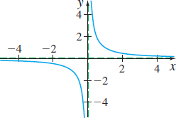
A change in concavity does not, of itself, guarantee an inflection point. For example, Figure 42 shows the graph of \(f(x)=\dfrac{1}{x}.\) The first and second derivatives are \(f^\prime (x) =-\dfrac{1}{x^{2}}\) and \(f^{\prime \prime} (x) =\dfrac{2}{x^{3}}\). Then \[ \hbox{ \(f^{\prime \prime} (x) =\dfrac{2}{x^{3}}<0\) if \(x<0\) and \(f^{\prime \prime}(x) =\dfrac{2}{x^{3}}>0\) if \(x>0\).} \]
So, \(f\) is concave down on \((-\infty ,0)\) and concave up on \(( 0,\infty )\), yet \(f\) has no inflection point at \(x=0\) because \(f\) is not defined at \(0\).
5 Use the Second Derivative Test to Find Local Extrema
291
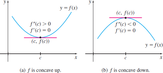
Suppose \(c\) is a critical number of \(f\) and \(f^\prime (c) =0\). This means that the graph of \(f\) has a horizontal tangent line at the point \((c,\;f(c))\). If \(f^{\prime \prime}\) exists on an open interval containing \(c\) and \(f^{\prime \prime} (c) >0\), then the graph of \(f\) is concave up on the interval, as shown in Figure 43(a). Intuitively, it would seem that \(f(c)\) is a local minimum value of \(f(c)\). If, on the other hand, \(f^{\prime \prime} (c) <0\), the graph of \(f\) is concave down on the interval, and \(f(c)\) would appear to be a local maximum value of \(f(c)\), as shown in Figure 43(b). The next theorem, known as the Second Derivative Test, confirms our intuition.
THEOREM Second Derivative Test
Let \(f\) be a function for which \(f^\prime\) and \(f^{\prime \prime}\) exist on an open interval \((a,b)\). Suppose \(c\) lies in \(( a,b)\) and is a critical number of \(f\):
- If \(f^{\prime \prime} (c) <0\), then \(f(c)\) is a local maximum value.
- If \(f^{\prime \prime} (c) >0\), then \(f(c)\) is a local minimum value.
Proof
Suppose \(f^{\prime \prime} (c) <0.\) Then \[ f^{\prime \prime} (c)=\lim\limits_{x\rightarrow c}\frac{f^\prime (x)-f^\prime (c)}{x-c}<0 \]
Now since \(\lim\limits_{x\rightarrow c}\dfrac{f^\prime (x)-f^\prime (c)}{x-c}<0\), there is an open interval about \(c\) for which \[ \frac{f^\prime (x)-f^\prime (c)}{x-c}<0 \]
everywhere in the interval, except possibly at \(c\) itself (refer to Example 7, p. 136, in Section 1.6). Since \(c\) is a critical number, \(f^\prime (c)=0\), so \[ \frac{f^\prime (x)}{x-c}<0 \]
For \(x<c\) on this interval, \(f^\prime (x)>0\), and for \(x>c\) on this interval, \(f^\prime (x)<0\). By the First Derivative Test, \(f(c)\) is a local maximum value.
In Problem 133, you are asked to prove that if \(f^{\prime \prime} (c) >0,\) then \(f(c)\) is a local minimum value.
Using the Second Derivative Test to Identify Local Extrema
- Determine where \(f(x)=x-2\cos x,\) \(0\) \(\leq x\leq 2\pi\), is concave up and concave down.
- Find any inflection points.
- Use the Second Derivative Test to identify any local extreme values.
292
Solution (a) Since \(f\) is continuous on the closed interval \([0,2\pi]\) and \(f^\prime\) and \(f^{\prime \prime}\) exist on the open interval \(\left( 0,\,2\pi \right)\), we can use the Test for Concavity. The first and second derivatives of \(f\) are \[ f^\prime (x) =\dfrac{d}{\textit{dx}}(x-2\;\cos x) =1+2\;\sin x \qquad \hbox{and}\qquad f^{\prime \prime} (x) =\dfrac{d}{\textit{dx}}(1+2\;\sin\;x) =2\;\cos x \]
To determine concavity, we solve the inequalities \(f^{\prime \prime} (x) <0\) and \(f^{\prime \prime} (x) >0.\) Since \(f^{\prime \prime} (x) =2\;\cos\;x,\) we have
- \(f^{\prime \prime} (x) > 0\qquad \hbox{ when }0<x<\dfrac{\pi }{2}\quad \hbox{ and }\quad\dfrac{3\pi }{2}<x<2\pi\)
- \(f^{\prime \prime} (x) < 0\qquad \hbox{ when }\dfrac{\pi }{2}<x<\dfrac{3\pi }{2}\)
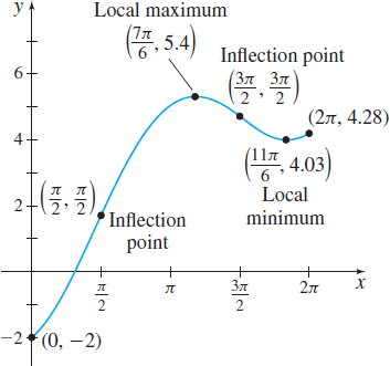
The function \(f\) is concave up on the intervals \(\left( 0,\dfrac{\pi }{2}\right)\) and \(\left( \dfrac{3\pi }{2},2\pi \right) ,\) and \(f\) is concave down on the interval \(\left( \dfrac{\pi }{2},\dfrac{3\pi }{2}\right)\).
(b) The concavity of \(f\) changes at \(\dfrac{\pi }{2}\) and \(\dfrac{3\pi }{2}\), so the points \(\left( \dfrac{\pi }{2},\dfrac{\pi }{2}\right)\) and \(\left( \dfrac{3\pi }{2},\dfrac{3\pi }{2}\right)\) are inflection points of \(f\).
(c) We find the critical numbers by solving the equation \(f^\prime(x) =0\). \[ \begin{eqnarray*} 1+2\;\sin\;x &=& 0\qquad 0\leq x\leq 2\pi \\ \sin\;x &=&-\dfrac{1}{2} \\ x=\frac{7\pi }{6}\qquad &&\hbox{ or }\qquad {x=\frac{11\pi }{6}} \end{eqnarray*} \]
Now using the Second Derivative Test, we get \[ f^{\prime \prime} \left(\dfrac{7\pi }{6}\right) =2\;\cos \left( \dfrac{7\pi }{6}\right) =- \sqrt{3}<0 \]
and \[ f^{\prime \prime} \left( \dfrac{11\pi }{6}\right) =2\;\cos \left(\dfrac{11\pi}{6}\right) = \sqrt{3}>0 \]
So, \[ f\left( \dfrac{7\pi }{6}\right) =\dfrac{7\pi }{6}-2\;\cos \dfrac{7\pi }{6}=\dfrac{7\pi }{6}+ \sqrt{3}\approx 5.4 \]
is a local maximum value, and \[ f\left( \dfrac{11\pi }{6}\right) =\dfrac{11\pi }{6}-2\cos \dfrac{11\pi }{6}=\dfrac{11\pi }{6}- \sqrt{3}\approx 4.03 \]
is a local minimum value.
See Figure 44 for the graph of \(f\).
NOW WORK
Problem 79.
If the second derivative of the function does not exist, the Second Derivative Test cannot be used. If the second derivative exists at a critical number, but equals \(0\) there, the Second Derivative Test gives no information. In these cases, the First Derivative Test must be used to identify local extreme points. An example is the function \(f(x)=x^{4}\). Both \(f^\prime (x) =4x^{3}\) and \(f^{\prime \prime} (x) =12x^{2}\) exist for all real numbers. Since \(f^\prime (0) =0\), \(0\) is a critical number of \(f\). But \(f^{\prime \prime} ( 0) =0\), so the Second Derivative Test gives no information about the behavior of \(f\) at \(0\).
293
Analyzing Monthly Sales
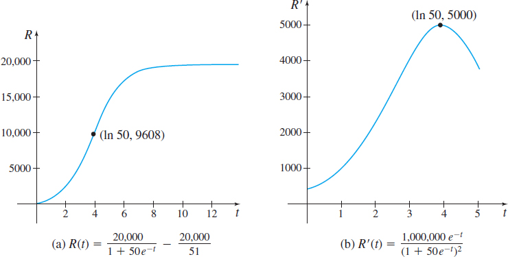
Unit monthly sales \(R\) of a new product over a period of time are expected to follow the logistic function \[ R=R(t) =\dfrac{20{,}000}{1+50e^{-t}}-\dfrac{20{,}000}{51}\qquad t\geq 0 \]
where \(t\) is measured in months.
- When are the monthly sales increasing? When are they decreasing?
- Find the rate of change of sales.
- When is the rate of change of sales \(R^\prime\) increasing? When is it decreasing?
- When is the rate of change of sales a maximum?
- Find any inflection points of \(R(t)\).
- Interpret the result found in (e).
Solution (a) We find \(R^\prime (t)\) and use the Increasing/Decreasing Function Test. \[ R^\prime (t) =\dfrac{d}{\textit{dt}}\left( \dfrac{20{,}000}{1+50e^{-t}}-\dfrac{20{,}000}{51}\right) =20{,}000\cdot \left[ \dfrac{50e^{-t}}{(1+50e^{-t}) ^{2}}\right] =\dfrac{1{,}000{,}000e^{-t}}{(1+50e^{-t}) ^{2}} \]
Since \(e^{-t}>0\) for all \(t\geq 0\), then \(R^\prime (t) >0\) for \(t\geq 0.\) The sales function \(R\) is an increasing function. So, monthly sales are always increasing.
(b) The rate of change of sales is given by the derivative \(R^\prime (t) =\dfrac{1{,}000{,}000e^{-t}}{(1+50e^{-t})^{2}},\) \(t\geq 0.\)
(c) Using the Increasing/Decreasing Function Test with \(R^\prime\), the rate of change of sales \(R^\prime\) is increasing when its derivative \(R^{\prime \prime} (t) >0;\) \(R^\prime (t)\) is decreasing when \(R^{\prime \prime} (t) <0\). \[ \begin{eqnarray*} R^{\prime \prime} (t) &=&\dfrac{d}{\textit{dt}}R^\prime (t) =1{,}000{,}000\left[ \dfrac{-e^{-t}(1+50e^{-t})^{2}+100e^{-2t}( 1+50e^{-t}) }{(1+50e^{-t})^{4}}\right] \\[12pt]&=&1{,}000{,}000e^{-t}\left[ \dfrac{-1-50e^{-t}+100e^{-t}}{(1+50e^{-t})^{3}}\right] =\dfrac{1{,}000{,}000e^{-t}}{(1+50e^{-t}) ^{3}}(50e^{-t}-1) \end{eqnarray*} \]
Since \(e^{-t}>0\) for all \(t\), the sign of \(R^{\prime \prime}\) depends on the sign of \(50e^{-t}-1\). \[ \begin{eqnarray*} \begin{array}{rl@{\qquad}rl} 50e^{-t}-1 &> 0 & 50e^{-t}-1 &<0\\[4pt] 50e^{-t} &> 1 & 50e^{-t} &<1 \\[4pt] 50 &> e^{t} & 50 &<e^{t} \\[4pt] t &< \ln 50 & t &>\ln 50 \end{array} \end{eqnarray*} \]
Since \(R^{\prime \prime} (t) >0\) for \(t<\ln 50 \approx 3.9\) and \(R^{\prime \prime} (t) <0\) for \(t>\ln 50 \approx 3.9\), the rate of change of sales is increasing for the first \(3.9\) months and is decreasing from \(3.9\) months on.
(d) The critical number of \(R^\prime\) is \(\ln 50 \approx 3.9\). Using the First Derivative Test, the rate of change of sales is a maximum about \(3.9\) months after the product is introduced.
(e) Since \(R^{\prime \prime} (t) >0\) for \(t<\ln 50\) and \(R^{\prime \prime} (t) <0\) for \(t>\ln 50\), the point \((\ln 50,9608)\) is the inflection point of \(R\).
(f) The sales function \(R\) is an increasing function, but at the inflection point \((\ln 50,9608)\) the rate of change in sales begins to decrease.
294
See Figure 45 for the graphs of \(R\) and \(R^\prime\).
NOW WORK
Problem 105.