CHAPTER 5 PROJECT
403
CHAPTER 5 PROJECT Managing the Klamath River

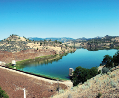
There is a gauge on the Klamath River, just downstream from the dam at Keno, Oregon. The U.S. Geological Survey has posted flow rates for this gauge every month since 1930. The averages of these monthly measurements since 1930 are given in Table 2. Notice that the data in Table 2 measure the rate of change of the volume \(V\) in cubic feet of water each second over one year; that is, the table gives \(\dfrac{dV}{dt}=V^\prime (t)\) in cubic feet per second, where \(t\) is in months.
Table 2: TABLE 2
| Month (t) | Flow Rate (\({ft}^{3}/{s}\)) |
|---|---|
| January (1) | 1911.79 |
| February (2) | 2045.40 |
| March (3) | 2431.73 |
| April (4) | 2154.14 |
| May (5) | 1592.73 |
| June (6) | 945.17 |
| July (7) | 669.46 |
| August (8) | 851.97 |
| September (9) | 1107.30 |
| October (10) | 1325.12 |
| November (11) | 1551.70 |
| December (12) | 1766.33 |
- Find the factor that will convert the data in Table 2 from seconds to days. [Hint: \(1\) day \(=1d =24 \hbox{ hours } =24h (60 min/h) = (24)(60 min\)) (\(60s/min\)).]
If we assume February has \(28.25\) days, to account for a leap year, then 1 year \(=365.25\) days. If \(V^\prime (t)\) is the rate of flow of water, in \(\hbox{cubic feet per day}\), the total flow of water over 1 year is given by \[ V=V(t) =\int_{0}^{365.25}V^\prime (t) dt. \] - Approximate the total annual flow using a Riemann sum. (Hint: Use \(\Delta t_{1}=31,\) \(\Delta t_{2}=28.25,\) etc.)
- The solution to Problem 2 finds the sum of \(12\) rectangles whose widths are \(\Delta t_{i},\) \(1\leq i\leq 12\), and whose heights are the flow rate for the \(i\)th month. Using the horizontal axis for time and the vertical axis for flow rate in ft\(^3\)/day, plot the points of Table 2 as follows: (January 1, flow rate for January), (February 1, flow rate for February)\(,\ldots ,\)(December 1, flow rate for December) and add the point (December 31, flow rate for January). Beginning with the point at January 1, connect each consecutive pair of points with a line segment, creating \(12\) trapezoids whose bases are \(\Delta t_{i}\), \(1\leq i\leq 12.\) Approximate the total annual flow \(V=V(t) =\int_{0}^{365.25}V^\prime (t)\, dt\) by summing the areas of these trapezoids.
- Using the horizontal axis for time and the vertical axis for flow rate in ft\(^3\)/day, plot the points of Table 2 as follows: (January 31, flow rate for January), (February 28, flow rate for February)\(,\ldots,\) (December 31, flow rate for December). Then add the point (January 1, flow rate for December) to the left of (January 31, flow rate for January). Connect consecutive points with a line segment, creating 12 trapezoids whose bases are \(\Delta t_{i},\) \(1\leq i\leq 12\). Approximate the total annual flow \(V=V(t) =\int_{0}^{365.25}V^\prime (t)\, dt\) by summing the areas of these trapezoids.
- Why did we add the extra point in Problems 3 and 4? How do you justify the choice?
- Compare the three approximations. Discuss which might be the most accurate.
- Consult Chapter 7 and read about Simpson's Rule (p. 514). Can you see a way to use it to approximate the total annual flow?
- Another way to approximate \(V=V(t) =\int_{0}^{365.25}V^\prime (t) dt\) is to fit a polynomial function to the data. We could find a polynomial of degree 11 that passes through every point of the data, but a polynomial of degree 6 is sufficient to capture the essence of the behavior. The polynomial function \(f\) of degree 6 is \[ \begin{eqnarray*} {f}(t) &=& 2.2434817\times 10^{-10}t^{6}-2.5288956\times 10^{-7}t^{5}\\ &+& 0.00010598313t^{4}- 0.019872628t^{3}+1.557403t^{2}\\ &-& 39.387734t+2216.2455 \end{eqnarray*} \] Find the total annual flow using \(f(t)=V^\prime (t)\).
 Use technology to graph the polynomial function \(f\) over the closed interval \([0,12] .\) How well does the graph fit the data?
- A manager could approximate the rate of flow of the river for every minute of every day using the function \[ \begin{eqnarray*} g(t)&=& 1529.403+510.330\sin \dfrac{2\pi t}{365.25}+489.377\cos \dfrac{2\pi t}{365.25}\\ &-& 47.049\sin \dfrac{4\pi t}{365.25}-249.059\cos \dfrac{4\pi t}{365.25} \end{eqnarray*} \] where \(t\) represents the day of the year in the interval \([0{,}365.25]\). The function \(g\) represents the best fit to the data that has the form of a sum of trigonometric functions with the period 1 year. We could fit the data perfectly using more terms, but the improvement in results would not be worth the extra work in handling that approximation. Use \(g\) to approximate the total annual flow.
- Use technology to graph the function \(g\) over the closed interval \([0,12]\). How well does the graph fit the data?
- Compare the five approximations to the annual flow of the river. Discuss the advantages and disadvantages of using one over another. What method would you recommend to measure the annual flow of the Klamath River?