6.5 Arc Length
OBJECTIVES
When you finish this section, you should be able to:
- Find the arc length of the graph of a function \({y\,=\,f(x)} \) (p. 439)
- Find the arc length of the graph of a function using a partition of the \( y\)-axis (p. 441)
We have already seen that a definite integral can be used to find the area of a plane region and the volume of certain solids. In this section, we will see that a definite integral can be used to find the length of a graph.
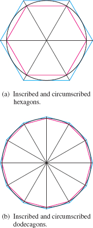
The idea of finding the length of a graph had its beginning with Archimedes. Ancient people knew that the ratio of the circumference \(C\) of any circle to its diameter \(d\) equaled the constant that we call \(\pi \). That is, \(\dfrac{C}{d}=\pi .\) But Archimedes is credited as being the first person to analytically investigate the numerical value of \(\pi\).* He drew a circle of diameter \(1\) unit, then inscribed (and circumscribed) the circle with regular polygons, and computed the perimeters of the polygons. He began with two hexagons (6 sides) and then two dodecagons (12 sides). See Figure 45. He continued until he had two polygons, each with 96 sides. He knew that the circumference \(C\) of the circle was larger than the perimeter of the inscribed polygon and smaller than the circumscribed polygon. In this way, he proved that \(3\dfrac{10}{71}<\pi < 3\dfrac{1}{7}.\) In essence, Archimedes approximated the length of the circle by representing it by smaller and smaller line segments and summing the lengths of the line segments.
439
Our approach to finding the length of the graph of a function is similar to that used by Archimedes and follows the ideas we used to find area and volume.
*Backmann, Peter, The History of \(\pi\). St Martin's Press, N.Y. 1971 p. 62.
1 Find the Arc Length of the Graph of a Function \(y=f(x) \)
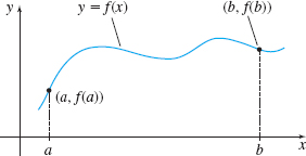
Suppose we want to find the length of the graph of a function \(y=f(x) \) from \(x=a\) to \(x=b\). We assume the derivative \(f' \) of \(f\) is continuous on some interval containing \(a\) and \(b\).* See Figure 46.
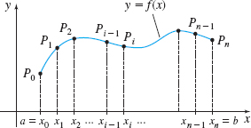
We begin by partitioning the closed interval \([a,b] \) into \(n\) subintervals: \begin{equation*} \lbrack a, x_{1}], [x_{1}, x_{2}], \ldots , [x_{i-1}, x_{i}], \ldots , [x_{n-1}, b]\qquad x_{0}=a\quad x_{n}=b \end{equation*}
each of width \(\Delta x=\dfrac{b-a}{n}\). Corresponding to each number \( a, x_{1}, x_{2},\ldots , x_{i-1}, x_{i}, \ldots , x_{n-1}, b\) in the partition, there are points \(P_{0}, P_{1}, P_{2}, \ldots ,\,P_{i-1},\,P_{i},\ldots , P_{n-1}, P_{n}\) on the graph of \(f\), as illustrated in Figure 47.
ORIGINS
Archimedes (287–212 BC) was a Greek astronomer, physicist, engineer, and mathematician. His contributions include the Archimedes screw, which is still used to lift water or grain, and the Archimedes principle, which states that the weight of an object can be determined by measuring the volume of water it displaces. Archimedes used the principle to measure the amount of gold in the king's crown; modern-day cooks can use it to measure the amount of butter to add to a recipe. Archimedes is also credited with using the Method of Exhaustion to find the area under a parabola and to approximate the value of \(\pi\).

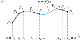
When each point \(P_{i-1}\) is connected to the next point \(P_{i}\) by a line segment, the sum \(L\) of the lengths of the line segments approximates the length of the graph of \(y=f(x)\) from \(x=a\) to \(x=b\). The sum \(L\) is given by \[ L=d( P_{0},P_{1}) +d( P_{1},P_{2}) +\cdots +d(P_{n-1},P_{n}) =\sum_{i=1}^{n}d( P_{i-1},P_{i}) \]
where \(d( P_{i-1},P_{i}) \) denotes the length of the line segment joining point \(P_{i-1}\) to point \(P_{i}\). See Figure 48.
NEED TO REVIEW?
The distance formula is discussed in Appendix A.3, p. A-16.
Using the distance formula, the length of the \(i\)th line segment is \begin{eqnarray*} d(P_{i-1},P_{i}) &=&\sqrt{(x_{i}-x_{i-1})^{2}+(y_{i}-y_{i-1})^{2}}= \sqrt{(\Delta x)^{2}+(\Delta y_{i})^{2}}\\[5pt] &=&\sqrt{\dfrac{( \Delta x) ^{2}+( \Delta y_{i}) ^{2}}{( \Delta x) ^{2}}}\cdot \sqrt{( \Delta x) ^{2}} \underset{\underset{\color{#0066A7}{\hbox{\(\Delta x > 0\)}}}{\color{#0066A7}{\uparrow }}} {=} \sqrt{1+\left( \frac{\Delta y_{i}}{\Delta x}\right) ^{2}} \Delta x\\[-11pt] \end{eqnarray*}
where \(\Delta x=\dfrac{b-a}{n}\) and \(\Delta y_{i}=y_{i}-y_{i-1}=f(x_{i})-f(x_{i-1})\). Then the sum of the lengths of the line segments is \begin{align*} \bbox[5px, border:1px solid black, #F9F7ED]{ L=\displaystyle \sum_{i=1}^{n}\left[ \sqrt{ 1+\left( \dfrac{\Delta y_{i}}{\Delta x}\right) ^{2}}~\Delta x\right] } \end{align*}
This sum is not a Riemann sum. To put this sum in the form of a Riemann sum, we need to express \(\sqrt{1+\left( \dfrac{\Delta y_{i}}{\Delta x}\right) ^{2} }\) in terms of \(u_{i},\) \(x_{i-1}\leq u_{i}\leq x_{i}.\) To do this, we first observe that the function \(f\) has a derivative \(f' \) that is continuous on an interval
440
NEED TO REVIEW?
The Mean Value Theorem is discussed in Section 4.3, pp. 276–279.
containing \(a\) and \(b\). It follows that \(f\) has a derivative on each subinterval \(( x_{i-1},x_{i}) \) of \(\left[ a,b \right] \). Now we use the Mean Value Theorem. Then in each open subinterval \(( x_{i-1}, x_{i}) \), there is a number \(u_{i}\) for which \begin{eqnarray*} f(x_{i})-f(x_{i-1}) &=&f'(u_{i})(x_{i}-x_{i-1}) & {\color{#0066A7}{\hbox{Apply the Mean Value Theorem.}}}\\ \Delta y_{i} &=&f'(u_{i})~\Delta x & {\color{#0066A7}{\Delta y_{i} =f(x_{i})-f(x_{i-1}); \Delta x=x_{i} -x_{i-1}.}}\\ \dfrac{\Delta y_{i}}{\Delta x} &=&f'(u_{i}) & {\color{#0066A7}{\hbox{Divide both sides by \(\Delta x\).}}} \end{eqnarray*}
Now the sum \(L\) of the lengths of the line segments can be written as \begin{align*} \bbox[5px, border:1px solid black, #F9F7ED]{L=\displaystyle \sum_{i=1}^{n}\Big[ \sqrt{1+[ f' (u_{i})] ^{2}}~\Delta x\Big] } \end{align*}
where \(u_{i}\) is some number in the open subinterval \((x_{i-1}, x_{i}) \).
This sum \(L\) is a Riemann sum. As the number of subintervals increases, that is, as \(n\rightarrow \infty \), the sum \(L\) becomes a better approximation to the arc length of the graph of \(y=f(x)\) from \(x=a\) to \(x = b\). Since \(f' \) is continuous on \([a,b] \), the limit is a definite integral.
Arc Length Formula
Suppose a function \(y=f(x) \) has a derivative that is continuous on an interval containing \(a\) and \(b\). The arc length \(s\) of the graph of \(~f\) from \(x=a\) to \(x=b\) is given by \begin{equation*} \bbox[5px, border:1px solid black, #F9F7ED]{ s=\int_{a}^{b}\sqrt{1+\left[ f' (x) \right] ^{2}}~{\it dx}}\tag{1} \end{equation*}
*We will discuss shortly the reason for this restriction.

Finding the Arc Length of a Graph
Find the arc length of the graph of the function \(f(x) =\ln~\sec~x\) from \(x=0\) to \(x=\dfrac{\pi}{4}\).
Solution The graph of \(f(x) =\ln~\sec~x\) is shown in Figure 49.
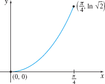
The derivative of \(f\) is \(f' (x)=\dfrac{\sec x\tan x}{\sec x}=\tan x\). Since \(f' (x) =\tan x\) is continuous on the open interval \(\left( -\dfrac{\pi}{2},\dfrac{\pi}{2} \right) ,\) which contains \(0\) and \( \dfrac{\pi}{4},\) we use the arc length formula (1). The arc length \(s\) from \(0\) to \(\dfrac{\pi}{4}\) is \begin{align*} s&=&\int_{0}^{\pi /4}\sqrt{~1+[ f' (x) ] ^{2}}~ {\it dx}=\int_{0}^{\pi /4}\sqrt{1+\tan ^{2}x}\,{\it dx}=\int_{0}^{\pi /4}\sqrt{\sec ^{2}x }\,{\it dx} \\[5pt] &=&\int_{0}^{\pi /4}\sec x\,{\it dx}=\big[ \ln \vert \sec x+\tan x\vert \big] _{0}^{\pi /4} \\[5pt] &=&\ln \left\vert \sec \dfrac{\pi}{4}+\tan \dfrac{\pi}{4}\right\vert -\ln \left\vert \sec 0+\tan 0\right\vert =\ln \vert \sqrt{2}+1\vert \end{align*}
Finding the Arc Length of a Graph
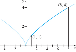
Find the arc length of the graph of the function \(f(x) =x^{2/3}\) from \(x=1\) to \(x=8\).
Solution We begin by graphing \(f(x) =x^{2/3}\). See Figure 50.
441
The derivative of \(f(x)=x^{2/3}\) is \(f' (x)=\dfrac{2}{3}x^{-1/3}=\dfrac{2}{3x^{1/3}}\). Notice that \(f' \) is not continuous at \(0\). However, since \(f'\) is continuous on an interval containing \(1\) and \( 8\) (use \(\left[ \dfrac{1}{2},9\right]\), for example, which avoids \(0)\), we use the arc length formula (1). The arc length \(s\) from \(x=1\) to \(x=8\) is \begin{eqnarray*} s&=&\int_{1}^{8}\sqrt{1+\left[ f' (x) \right] ^{2}} ~{\it dx}=\int_{1}^{8}\sqrt{1+\left( \frac{2}{3x^{1/3}}\right) ^{2}} ~{\it dx}=\int_{1}^{8}\sqrt{1+\frac{4}{9x^{2/3}}}~{\it dx} \\[5pt] &=&\int_{1}^{8}\sqrt{\frac{9x^{2/3}+4}{9x^{2/3}}}~{\it dx} \underset{\underset{\underset{\color{#0066A7}{\hbox{so \(\sqrt{x^{2/3}} =x^{1/3}\)}}}{\color{#0066A7}{\hbox{\(x>0\) on \([1,8]\),}}}} {\color{#0066A7}{\uparrow }}} {=} {\frac{1}{3}} \int_{1}^{8}\Big( x^{-1/3}\sqrt{9x^{2/3}+4}\Big) ~{\it dx}\\[-9pt] \end{eqnarray*}
We use the substitution \(u=9x^{2/3}+4.\) Then \({\it du}=6x^{-1/3}{\it dx}\) and, \( x^{-1/3}{\it dx}=\dfrac{{\it du}}{6}\). The limits of integration change to \(u=13\) when \(x=1\), and to \(u=40\) when \(x=8\). Then \begin{eqnarray*} s&=&\dfrac{1}{3} \displaystyle \int_{1}^{8}\Big[ x^{-1/3}\sqrt{~9x^{2/3}+4}\Big] ~{\it dx}= \dfrac{1}{3}\displaystyle \int_{13}^{40}\sqrt{~u}~\dfrac{{\it du}}{6}= \dfrac{1}{18} \left[\dfrac{u^{3/2}}{\dfrac{3}{2}}\right] _{13}^{40}\\[5pt] &=&\dfrac{1}{27}\big( 80\sqrt{10}-13\sqrt{13}\big) \end{eqnarray*}
NOW WORK
Problem 9.
2 Find the Arc Length of the Graph of a Function Using a Partition of the \(y\)-Axis
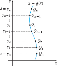
For a function defined by \(x=g(y),\) where \(g'\) is continuous on an open interval containing the numbers \(c\) and \(d,\) we can find the arc length of the graph of \(g\) from \(y=c\) to \(y=d\) by using a partition of the \(y\)-axis. We begin by partitioning the interval \([c,d]\) into \(n\) subintervals: \begin{equation*} [ c,y_{1}] , [ y_{1},y_{2}] , \ldots , [ y_{i-1},y_{i}] , \ldots , [ y_{n-1},d]\qquad y_{0}=c\quad y_{n}=d \end{equation*}
each of width \(\Delta y=\frac{d-c}{n}\). Corresponding to each number \(c, y_{1}, y_{2}, \ldots, y_{i-1}, y_{i}, \ldots , y_{n-1}, d\), there are points \(Q_{0}, Q_{1}, Q_{2}, \ldots , Q_{i-1}, Q_{i}, \ldots , Q_{n-1}, Q_{n}\) on the graph of \(g\), as shown in Figure 51. By forming line segments connecting each point \(Q_{i-1}\) to \(Q_{i}\), for \(i=1,2,3,\ldots ,n,\) and following the same process as described for a partition of the \(x\)-axis, we obtain the following result:
Arc Length
For a function defined by \(x=g(y),\) where \(g'\) is continuous on an interval containing \(c\) and \(d\), the arc length \(s\) of the graph of \(g\) from \(y=c\) to \(y=d\) is given by \begin{equation} \bbox[5px, border:1px solid black, #F9F7ED]{s= \int_{c}^{d}\sqrt{1+[g'(y)]^{2}}{\it dy} }\notag\tag{2} \end{equation}
The result in (2) can sometimes be used to find the length of the graph of a function \(y=f(x)\) from \(a\) to \(b\) when its derivative \(f'\) is not continuous at some number in \([a,b].\)
Finding the Arc Length of a Function
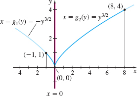
Find the arc length of \(f(x) =x^{2/3}\) from \(x=-1\) to \(x=8.\)
Solution Since the derivative \(f'(x) =\dfrac{2}{3x^{1/3}}\) does not exist at \(x=0\), we cannot use the arc length formula (1) to find the length of the graph from \(x=-1\) to \(x=8.\)
442
From Figure 52, we observe that the length of the graph of \(f\) from \(x=-1\) to \(x=8\) is the same as the length of the graph of \(x=g_{1}( y) =-y^{3/2}\) from \(y=0\) to \(y=1\) plus the length of the graph of \(x=g_{2}( y) =y^{3/2}\) from \(y=0\) to \(y=4.\)
We investigate \(x=g_{1}(y) =-y^{3/2}\) first. Since \(g_{1}' (y) =-\dfrac{3}{2}y^{1/2}\) is continuous for all \(y\geq 0.\) we can use arc length formula (2) to find the arc length \(s_{1}\) of \(g_{1}\) from \(y=0\) to \(y=1\). \begin{eqnarray*} s_{1}&=&\int_{0}^{1}\sqrt{1+[g_{1}'(y)]^{2}}{\it dy} \underset{\underset{\color{#0066A7}{\hbox{\(g_{1}'(y)\)} =-\frac{3}{2}y^{1/2}}}{\color{#0066A7}{\uparrow }}}{=}\int_{0}^{1} \sqrt{1+\left(\frac{3}{2}y^{1/2}\right) ^{2}}~{\it dy}\\[-11pt] &=&\int_{0}^{1}\sqrt{1+ \frac{9}{4}y}~{\it dy}=\frac{1}{2}\int_{0}^{1}\sqrt{4+9y}~{\it dy} \end{eqnarray*}
We use the substitution \(u=4+9y\). Then \({\it du}=9~{\it dy}\) or, equivalently, \({\it dy}= \dfrac{{\it du}}{9}\). The limits of integration are \(u=4\) when \(y=0\), and \(u=13\) when \(y=1.\) \begin{equation*} s_{1}=\frac{1}{2}\displaystyle \int_{4}^{13}\sqrt{u}~\frac{{\it du}}{9}=\frac{1}{18}\left[ \frac{u^{3/2}}{\dfrac{3}{2}}\right] _{4}^{13}=\frac{1}{27}\big( 13\sqrt{13}-8\big) \end{equation*}
Now we investigate \(x=g_{2}(y)\). Since \(g_{2}' (y) =\dfrac{3}{2}y^{1/2}\) is continuous for all \(y\geq 0,\) we can use arc length formula (2) to find the arc length \(s_{2}\) of \(g_{2}\) from \(y=0\) to \(y=4\). \[ \begin{array}{rcl@{\qquad}l} s_{2} &=&\int_{0}^{4}\sqrt{1+[g_{2}'(y)] ^{2}}~{\it dy}=\int_{0}^{4}\sqrt{1+\left(\dfrac{3}{2}y^{1/2}\right)^{~2}} ~{\it dy}\\ &=&\int_{0}^{4}\sqrt{1+\dfrac{9}{4}y}~{\it dy} =\frac{1}{2}\int_{0}^{4}\sqrt{4+9y}~{\it dy} &\color{#0066A7}{\hbox{Let \(u=4+9y \); }}\\ &&&\color{#0066A7}{\hbox{\(du=9dy \).}}\\ &=&\frac{1}{2}\int_{4}^{40}\sqrt{u}~\frac{{\it du}}{9}=\frac{1}{18}\left[ \frac{u^{3/2}}{\frac{3}{2}}\right] _{4}^{40}=\frac{1}{27}\big( 80\sqrt{10}-8\big) \end{array}\]
The arc length \(s\) of \(y=f(x) =x^{2/3}\) from \(x=-1\) to \(x=8\) is the sum \begin{eqnarray*} s&=&s_{1}+s_{2}=\frac{1}{27}\big( 13\sqrt{13}-8\big) +\dfrac{1}{27}\big( 80\sqrt{10}-8\big)\\[4pt] &=&\frac{1}{27} \big( 80\sqrt{10}+13\sqrt{13}-16\big) \end{eqnarray*}
NOW WORK
Problem 23.