11.1 Parametric Equations
Imagine a particle moving along a curve \(C\) in the plane as in Figure 11.1. We can describe the particle’s motion by specifying its coordinates as functions of time \(t\): \[ \boxed{\bbox[#fef7e5,5pt]{ x=f(t),\qquad y=g(t)}}\tag{1} \]
Note
We use the term “particle” when we treat an object as a moving point, ignoring its internal structure.
In other words, at time \(t\), the particle is located at the point \[\boxed{\bbox[#fef7e5,5pt]{ c(t)=(f(t),g(t))}} \]
The equations (1) are called parametric equations, and \(C\) is called a parametric curve. We refer to \(c(t)\) as a parametrization with parameter \(t\).
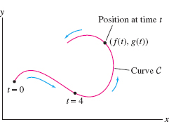
Because \(x\) and \(y\) are functions of \(t\), we often write \(c(t)=(x(t),y(t))\) instead of \((f(t),g(t))\). Of course, we are free to use any variable for the parameter (such as \(s\) or \(\theta\)). In plots of parametric curves, the direction of motion is often indicated by an arrow as in Figure 11.1.
608
EXAMPLE 1
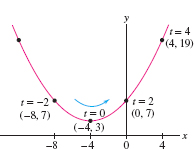
Sketch the curve with parametric equations \[ x = 2t-4,\qquad y = 3+t^2\tag{2} \]
Solution First compute the \(x\)- and \(y\)-coordinates for several values of \(t\) as in Table 11.1, and plot the corresponding points \((x,y)\) as in Figure 11.2. Then join the points by a smooth curve, indicating the direction of motion with an arrow.
| \(t\) | \(x=2t-4\) | \(y=3+t^2\) |
| \(-2\) | \(-8\) | 7 |
| 0 | \(-4\) | 3 |
| 2 | 0 | 7 |
| 4 | 4 | 19 |
CONCEPTUAL INSIGHT
The graph of a function \(y=f(x)\) can always be parametrized in a simple way as \[ c(t)=(t,f(t)) \]
For example, the parabola \(y=x^2\) is parametrized by \(c(t) = (t,t^2)\) and the curve \(y = e^t\) by \(c(t) = (t,e^t)\). An advantage of parametric equations is that they enable us to describe curves that are not graphs of functions. For example, the curve in Figure 11.3 is not of the form \(y=f(x)\) but it can be expressed parametrically.
As we have just noted, a parametric curve \(c(t)\) need not be the graph of a function. If it is, however, it may be possible to find the function \(f(x)\) by “eliminating the parameter” as in the next example.
EXAMPLE 2 Eliminating the Parameter
Describe the parametric curve \[ c(t) = (2t- 4,3+t^2) \] of the previous example in the form \(y=f(x)\).
Solution We “eliminate the parameter” by solving for \(y\) as a function of \(x\). First, express \(t\) in terms of \(x\): Since \(x = 2t-4\), we have \(t = \frac12x+ 2\). Then substitute \[ y = 3+t^2 = 3+\left(\frac12x+ 2\right)^2 = 7+2x +\frac14x^2 \]
Thus, \(c(t)\) traces out the graph of \(f(x) =7+2x +\frac14x^2\) shown in Figure 11.2.
EXAMPLE 3
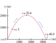
A bullet follows the trajectory \[ c(t) = (80t, 200t-4.9t^2) \] until it hits the ground, with \(t\) in seconds and distance in meters (Figure 11.4). Find:
- (a) The bullet’s height at \(t=5\) s.
- (b) Its maximum height.
609
Solution The height of the bullet at time \(t\) is \(y(t) = 200t - 4.9t^2\).
CAUTION
The graph of height versus time for an object tossed in the air is a parabola (by Galileo’s formula). But keep in mind that Figure 11.4 is not a graph of height versus time. It shows the actual path of the bullet (which has both a vertical and a horizontal displacement).
- (a) The height at \(t=5\) s is \[ y(5) = 200(5)-4.9(5^2) = 877.5 \mathrm{m} \]
- (b) The maximum height occurs at the critical point of \(y(t)\): \[ y'(t) =\frac{d}{dx}{t}(200t - 4.9t^2) = 200 - 9.8t = 0\quad\Rightarrow\quad t = \frac{200}{9.8}\approx 20.4 \,\,\mathrm{s} \]
The bullet’s maximum height is \(y(20.4) = 200(20.4) - 4.9(20.4)^2 \approx 2041 \mathrm{m}\).
We now discuss parametrizations of lines and circles. They will appear frequently in later chapters.
THEOREM 1 Parametrization of a Line
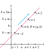
(a) The line through \(P=(a,b)\) of slope \(m\) is parametrized by \[ \boxed{\bbox[#fef7e5,5pt]{ x = a+rt,\qquad y = b+st \qquad -\infty < t < \infty}}\tag{3} \] for any \(r\) and \(s\) (with \(r\ne 0\)) such that \(m=s/r\).
(b) The line through \(P=(a,b)\) and \(Q= (c,d)\) has parametrization \[ \boxed{\bbox[#fef7e5,5pt]{ x = a +t(c-a),\qquad y = b + t(d-b)\qquad -\infty < t < \infty}}\tag{4} \] The segment from \(P\) to \(Q\) corresponds to \(0\le 1\le t\).
Solution (a) Solve \(x = a+rt\) for \(t\) in terms of \(x\) to obtain \(t = (x-a)/r\). Then \[ y = b+st = b +s\left(\frac{x-a}r\right) = b+m(x-a) \qquad\textrm{or}\qquad y-b=m(x-a) \] This is the equation of the line through \(P=(a,b)\) of slope \(m\). The choice \(r=1\) and \(s=m\) yields the parametrization in Figure 11.5.
The parametrization in (b) defines a line that satisfies \((x(0),y(0))=(a,b)\) and \((x(1),y(1))=(c,d)\). Thus, it parametrizes the line through \(P\) and \(Q\) and traces the segment from \(P\) to \(Q\) as \(t\) varies from \(0\) to \(1\).
EXAMPLE 4 Parametrization of a Line
Find parametric equations for the line through \(P=(3,-1)\) of slope \(m=4\).
Solution We can parametrize the line by taking \(r=1\) and \(s=4\) in Eq. (3): \[ x = 3+t, \qquad y = -1+4t \]
This is also written as \(c(t) = (3+t, -1+4t)\). Another parametrization of the line is \(c(t) = (3+5t, -1+20t)\), corresponding to \(r=5\) and \(s=20\) in Eq. (3).
610
The circle of radius \(R\) centered at the origin has the parametrization \[ x = R\cos\theta,\qquad y = R\sin\theta \]
The parameter \(\theta\) represents the angle corresponding to the point \((x,y)\) on the circle (Figure 11.6). The circle is traversed once in the counterclockwise direction as \(\theta\) varies over a half-open interval of length \(2\pi\) such as \([0,2\pi)\) or \([-\pi,\pi)\).
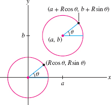
More generally, the circle of radius \(R\) with center \((a,b)\) has parametrization (Figure 11.6) \[ \boxed{\bbox[#fef7e5,5pt]{ x = a + R\cos \theta,\qquad y = b+R\sin \theta}}\tag{5} \]
As a check, let’s verify that a point \((x,y)\) given by Eq. (5) satisfies the equation of the circle of radius \(R\) centered at \((a,b)\): \begin{align*} (x-a)^2+(y-b)^2 &= (a + R\cos \theta-a)^2+(b+R\sin \theta-b)^2\\ & = R^2\cos^2\theta + R^2\sin^2\theta =R^2 \end{align*}
In general, to translate (meaning “to move”) a parametric curve horizontally \(a\) units and vertically \(b\) units, replace \(c(t)=(x(t),y(t))\) by \(c(t)=(a+x(t),b+y(t))\).
Suppose we have a parametrization \(c(t) = (x(t), y(t))\) where \(x(t)\) is an even function and \(y(t)\) is an odd function, that is, \(x(-t)=x(t)\) and \(y(-t)=-y(t)\). In this case, \(c(-t)\) is the reflection of \(c(t)\) across the \(x\)-axis: \[c(-t) = (x(-t), y(-t)) = (x(t), -y(t))\]
The curve, therefore, is symmetric with respect to the \(x\)-axis. We apply this remark in the next example and in Example 7 below.
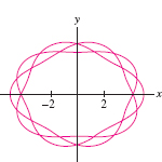
EXAMPLE 5 Parametrization of an Ellipse
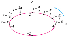
Verify that the ellipse with equation \(\big(\tfrac{x}a\big)^2+\big(\tfrac{y}b\big)^2=1\) is parametrized by \[ \boxed{\bbox[#fef7e5,5pt]{ c(t) = (a\cos t,\,b\sin t) \qquad\quad \textrm{(for \(-\pi\le t <\pi\))}}} \] Plot the case \(a= 4\), \(b=2\).
Solution To verify that \(c(t)\) parametrizes the ellipse, show that the equation of the ellipse is satisfied with \(x = a\cos t\), \(y = b\sin t\): \[ \left(\frac{x}a\right)^2 + \left(\frac{y}b\right)^2 = \left(\frac{a\cos t}a\right)^2 + \left(\frac{b\sin t}b\right)^2 = \cos^2t+\sin^2t = 1 \]
To plot the case \(a= 4\), \(b=2\), we connect the points corresponding to the \(t\)-values in Table 11.2 (see Figure 11.7). This gives us the top half of the ellipse corresponding to \(0\le t\le \pi\). Then we observe that \(x(t)=4\cos t\) is even and \(y(t) = 2\sin t\) is odd. As noted above, this tells us that the bottom half of the ellipse is obtained by symmetry with respect to the \(x\)-axis.
| \(t\) | \(x(t)=4\cos t\) | \(y(t)=2\sin t\) |
| \(0\) | \(4\) | \(0\) |
| \(\dfrac{\pi}6\) | \(2\sqrt 3\) | \(1\) |
| \(\dfrac{\pi}3\) | \(2\) | \(\sqrt 3\) |
| \(\dfrac{\pi}{2}\) | \(0\) | \(2\) |
| \(\dfrac{2\pi}{3}\) | \(-2\) | \(\sqrt{3}\) |
| \(\dfrac{5\pi}{6}\) | \(-2\sqrt{3}\) | \(1\) |
| \(\dfrac{\pi}{2}\) | \(-4\) | \(0\) |
611
A parametric curve \(c(t)\) is also called a path. This term emphasizes that \(c(t)\) describes not just an underlying curve \(C\), but a particular way of moving along the curve.
CONCEPTUAL INSIGHT
The parametric equations for the ellipse in Example 5 illustrate a key difference between the path \(c(t)\) and its underlying curve \(C\). The curve \(C\) is an ellipse in the plane, whereas \(c(t)\) describes a particular, counterclockwise motion of a particle along the ellipse. If we let \(t\) vary from \(0\) to \(4\pi\), then the particle goes around the ellipse twice.
A key feature of parametrizations is that they are not unique. In fact, every curve can be parametrized in infinitely many different ways. For instance, the parabola \(y=x^2\) is parametrized not only by \((t,t^2)\) but also by \((t^3,t^6)\), or \((t^5,t^{10})\), and so on.
EXAMPLE 6 Different Parametrizations of the Same Curve
Describe the motion of a particle moving along each of the following paths.
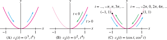
- (a) \(c_1(t) = (t^3, t^6)\)
- (b) \(c_2(t) = (t^2, t^4)\)
- (c) \(c_3(t) = (\cos t, \cos^2t)\)
Solution Each of these parametrizations satisfies \(y=x^2\), so all three parametrize portions of the parabola \(y=x^2\).
- (a) As \(t\) varies from \(-\infty\) to \(\infty\), the function \(t^3\) also varies from \(-\infty\) to \(\infty\). Therefore, \(c_1(t) = (t^3, t^6)\) traces the entire parabola \(y=x^2\), moving from left to right and passing through each point once [Figure 11.8].
- (b) Since \(x = t^2 \ge 0\), the path \(c_2(t) = (t^2, t^4)\) traces only the right half of the parabola. The particle comes in toward the origin as \(t\) varies from \(-\infty\) to \(0\), and it goes back out to the right as \(t\) varies from \(0\) to \(\infty\) [Figure 11.8].
- (c) As \(t\) varies from \(-\infty\) and \(\infty\), \(\cos t\) oscillates between 1 and \(-1\). Thus a particle following the path \(c_3(t) = (\cos t, \cos^2t)\) oscillates back and forth between the points \((1,1)\) and \((-1,1)\) on the parabola. [Figure 11.8].
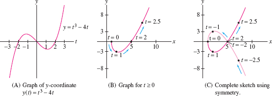
EXAMPLE 7 Using Symmetry to Sketch a Loop
Sketch the curve \[ c(t) = (t^2+1, t^3-4t) \] Label the points corresponding to \(t = 0, \pm 1, \pm 2, \pm 2.5\).
Solution
Step 1. Use symmetry.
Observe that \(x(t) = t^2+1\) is an even function and that \(y(t)=t^3-4t\) is an odd function. As noted before Example 5, this tells us that \(c(t)\) is symmetric with respect to the \(x\)-axis. Therefore, we will plot the curve for \(t\ge 0\) and reflect across the \(x\)-axis to obtain the part for \(t\le 0\).
612
Step 2. Analyze \(x(t)\), \(y(t)\) as functions of \(t\)
We have \(x(t)= t^2 +1\) and \(y(t) = t^3 -4t\). The \(x\)-coordinate \(x(t) = t^2+1\) increases to \(\infty\) as \(t\to \infty\). To analyze the \(y\)-coordinate, we graph \(y(t)=t^3-4t= t(t-2)(t+2)\) as a function of \(t\) (not as a function of \(x\)). Since \(y(t)\) is the height above the \(x\)-axis, Figure 11.9 shows that \begin{alignat*}{4} y(t)&<0& \qquad&\textrm{for}&\qquad &0 < t < 2,&\quad&\Rightarrow\quad\textrm{curve below \(x\)-axis}\\ y(t)&>0& \qquad &\textrm{for}&\qquad &t > 2,&\quad&\Rightarrow\quad\textrm{curve above \(x\)-axis} \end{alignat*}
So the curve starts at \(c(0)=(1,0)\), dips below the \(x\)-axis and returns to the \(x\)-axis at \(t=2\). Both \(x(t)\) and \(y(t)\) tend to \(\infty\) as \(t \to \infty\). The curve is concave up because \(y(t)\) increases more rapidly than \(x(t)\).
Step 3. Plot points and join by an arc.
The points \(c(0)\), \(c(1)\), \(c(2)\), \(c(2.5)\) tabulated in Table 11.3 are plotted and joined by an arc to create the sketch for \(t\ge 0\) as in Figure 11.9. The sketch is completed by reflecting across the \(x\)-axis as in Figure 11.9.
| \(t\) | \(x = t^2+1\) | \(y = t^3-4t\) |
| 0 | 1 | 0 |
| 1 | 2 | \(-3\) |
| 2 | 5 | 0 |
| 2.5 | 7.25 | 5.625 |
A cycloid is a curve traced by a point on the circumference of a rolling wheel as in Figure 11.10. Cycloids are famous for their “brachistochrone property” (see the marginal note below).
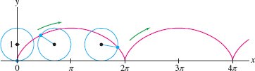
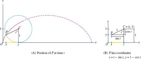
EXAMPLE 8 Parametrizing the Cycloid
Find parametric equations for the cycloid generated by a point \(P\) on the unit circle.
Note
A stellar cast of mathematicians (including Galileo, Pascal, Newton, Leibniz, Huygens, and Bernoulli) studied the cycloid and discovered many of its remarkable properties. A slide designed so that an object sliding down (without friction) reaches the bottom in the least time must have the shape of an inverted cycloid. This is the brachistochrone property, a term derived from the Greek brachistos, “shortest,” and chronos, “time.”
Solution The point \(P\) is located at the origin at \(t=0\). At time \(t\), the circle has rolled \(t\) radians along the \(x\) axis and the center \(C\) of the circle then has coordinates \((t,1)\) as in Figure 11.11. Figure 11.11 shows that we get from \(C\) to \(P\) by moving down \(\cos t\) units and to the left \(\sin t\) units, giving us the parametric equations \[ \boxed{\bbox[#fef7e5,5pt]{ x(t) = t - \sin t,\qquad y(t) = 1 - \cos t}}\tag{5} \]
613
The argument in Example 8 shows in a similar fashion that the cycloid generated by a circle of radius \(R\) has parametric equations \[ \boxed{\bbox[#fef7e5,5pt]{x = Rt - R\sin t,\qquad y= R - R\cos t}}\tag{6} \]
Next, we address the problem of finding tangent lines to parametric curves. The slope of the tangent line is the derivative \(dy/dx\), but we have to use the Chain Rule to compute it because \(y\) is not given explicitly as a function of \(x\). Write \(x = f(t)\), \(y = g(t)\). Then, by the Chain Rule in Leibniz notation, \[ g'(t) = \frac{dy}{dt} = \frac{dy}{dx}\,\frac{dx}{dt}= \frac{dy}{dx}\,f'(t) \]
If \(f'(t)\ne 0\), we can divide by \(f'(t)\) to obtain \[ \frac{dy}{dx} = \frac{g'(t)}{f'(t)} \]
Notation
In this section, we write \(f'(t), x'(t), y'(t)\), and so on to denote the derivative with respect to \(t\).
This calculation is valid if \(f(t)\) and \(g(t)\) are differentiable, \(f'(t)\) is continuous, and \(f'(t)\ne 0\). In this case, the inverse \(t=f^{-1}(x)\) exists, and the composite \(y=g(f^{-1}(x))\) is a differentiable function of \(x\).
Caution
Do not confuse \(dy/dx\) with the derivatives \(dx/dt\) and \(dy/dt\), which are derivatives with respect to the parameter \(t\). Only \(dy/dx\) is the slope of the tangent line.
THEOREM 2 Slope of the Tangent Line
Let \(c(t) = (x(t),y(t))\), where \(x(t)\) and \(y(t)\) are differentiable. Assume that \(x'(t)\) is continuous and \(x'(t)\ne 0\). Then \[ \boxed{\bbox[#fef7e5,5pt]{\frac{dy}{dx} = \frac{dy/dt}{dx/dt} =\frac{y'(t)}{x'(t)}}}\tag{7} \]
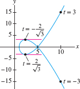
EXAMPLE 9
Let \(c(t) = (t^2+1, t^3-4t)\). Find:
- (a) An equation of the tangent line at \(t =3\)
- (b) The points where the tangent is horizontal (Figure 11.12).
Solution We have \[ \frac{dy}{dx} = \frac{y'(t)}{x'(t)} = \frac{(t^3-4t)'}{(t^2+1)'} = \frac{3t^2-4}{2t} \]
614
(a) The slope at \(t = 3\) is \[ \frac{dy}{dx} =\frac{3t^2-4}{2t}\bigg|_{t=3} = \frac{3(3)^2-4}{2(3)}= \frac{23}6 \]
Since \(c(3) = (10,15)\), the equation of the tangent line in point-slope form is \[ y - 15 = \frac{23}{6}(x-10) \]
(b) The slope \(dy/dx\) is zero if \(y'(t)=0\) and \(x'(t)\ne 0\). We have \(y'(t)=3t^2-4=0\) for \(t = \pm 2/\sqrt{3}\) (and \(x'(t)=2t \neq 0\) for these values of \(t\)). Therefore, the tangent line is horizontal at the points \[ c\left(-\frac{2}{\sqrt 3}\right) = \left(\frac73, \frac{16}{3\sqrt 3}\right),\qquad c\left(\frac{2}{\sqrt 3}\right) = \left(\frac73, -\frac{16}{3\sqrt 3}\right) \]
Note
Bézier curves were invented in the 1960s by the French engineer Pierre Bézier (1910–1999), who worked for the Renault car company. They are based on the properties of Bernstein polynomials, introduced 50 years earlier by the Russian mathematician Sergei Bernstein to study the approximation of continuous functions by polynomials. Today, Béezier curves are used in standard graphics programs, such as Adobe Illustrator\(^{\scriptscriptstyle\mathsf{TM}}\) and Corel Draw\(^{\scriptscriptstyle\mathsf{TM}}\), and in the construction and storage of computer fonts such as TrueType\(^{\scriptscriptstyle\mathsf{TM}}\) and PostScript\(^{\scriptscriptstyle\mathsf{TM}}\) fonts.
Parametric curves are widely used in the field of computer graphics. A particularly important class of curves are Bézier curves, which we discuss here briefly in the cubic case. Given four “control points” (Figure 11.13): \[ P_0=(a_0,b_0),\qquad P_1=(a_1,b_1),\qquad P_2=(a_2,b_2),\qquad P_3=(a_3,b_3) \] the Bézier curve \(c(t) = (x(t), y(t))\) is defined for \(0\le t \le 1\) by \begin{align} \label{12.param.bezx} x(t) & a_0(1-t)^3+3a_1t(1-t)^2+3a_2t^2(1-t) +a_3t^3\tag{8}\\ y(t) &= b_0(1-t)^3+3b_1t(1-t)^2+3b_2t^2(1-t) +b_3t^3\tag{9} \label{12.param.bezy} \end{align}
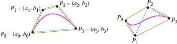
Note that \(c(0)=(a_0,b_0)\) and \(c(1)=(a_3,b_3)\), so the Bézier curve begins at \(P_0\) and ends at \(P_3\) (Figure 11.13). It can also be shown that the Bézier curve is contained within the quadrilateral (shown in blue) with vertices \(P_0, P_1, P_2, P_3\). However, \(c(t)\) does not pass through \(P_1\) and \(P_2\). Instead, these intermediate control points determine the slopes of the tangent lines at \(P_0\) and \(P_3\), as we show in the next example (also, see Exercises 65–68).
EXAMPLE 10
Show that the Bézier curve is tangent to segment \(\overline{P_0P_1}\) at \(P_0\).
Solution The Bézier curve passes through \(P_0\) at \(t = 0\), so we must show that the slope of the tangent line at \(t=0\) is equal to the slope of \(\overline{P_0P_1}\). To find the slope, we compute the derivatives: \begin{align*} x'(t) &= -3a_0(1-t)^2+ 3a_1(1-4t+3t^2)+a_2(2t-3t^2) +3a_3t^2\\ y'(t) &= -3b_0(1-t)^2+3b_1(1-4t+3t^2)+b_2(2t-3t^2) +3b_3t^2 \end{align*}
Evaluating at \(t=0\), we obtain \(x'(0)=3(a_1-a_0)\), \(y'(0)=3(b_1-b_0)\), and \[ \frac{dy}{dx}\bigg|_{t=0} =\frac{y'(0)}{x'(0)} = \frac{3(b_1-b_0)}{3(a_1-a_0)}= \frac{b_1-b_0}{a_1-a_0} \]
This is equal to the slope of the line through \(P_0=(a_0,b_0)\) and \(P_1=(a_1,b_1)\) as claimed (provided that \(a_1 \neq a_0\)).
11.1.1 Summary
615
- A parametric curve \(c(t) = (f(t), g(t))\) describes the path of a particle moving along a curve as a function of the parameter \(t\).
- Parametrizations are not unique: Every curve \(C\) can be parametrized in infinitely many ways. Furthermore, the path \(c(t)\) may traverse all or part of \(C\) more than once.
- Slope of the tangent line at \(c(t)\): \[ \frac{dy}{dx} = \frac{dy/dt}{dx/dt} = \frac{y'(t)}{x'(t)} \qquad\quad \textrm{(valid if \(x'(t)\ne 0\))} \]
- Do not confuse the slope of the tangent line \(dy/dx\) with the derivatives \(dy/dt\) and \(dx/dt\), with respect to \(t\).
- Standard parametrizations:
- – Line of slope \(m=s/r\) through \(P=(a,b)\): \(c(t) = (a+rt,b+st)\).
- – Circle of radius \(R\) centered at \(P=(a,b)\): \(c(t) = (a+R\cos t, b+R\sin t)\).
- – Cycloid generated by a circle of radius \(R\): \(c(t) = (R(t-\sin t), R(1-\cos t))\).