1.1 Real Numbers, Functions, and Graphs
We begin with a short discussion of real numbers. This gives us the opportunity to recall some basic properties and standard notation.
A real number is a number represented by a decimal or “decimal expansion.” There are three types of decimal expansions: finite, repeating, and infinite but nonrepeating. For example,
\begin{gather*} \frac{3}{8}=0.375,\quad \frac{1}{7}=0.142857142857\ldots=0.\overline{142857}\\ \pi = 3.141592653589793\ldots \end{gather*}
The number \(\frac{3}{8}\) is represented by a finite decimal, whereas \(\frac{1}{7}\) is represented by a repeating or periodic decimal. The bar over \(142857\) indicates that this sequence repeats indefinitely. The decimal expansion of \(\pi\) is infinite but nonrepeating.
The set of all real numbers is denoted by a boldface \(\mathbb{R}\). When there is no risk of confusion, we refer to a real number simply as a number. We also use the standard symbol \(\in\) for the phrase “belongs to.” Thus,
\[ a\in\mathbb{R}\quad\text{reads}\quad\unicode{8220} \text{\(a\) belongs to \(\mathbb{R}\)}\unicode{8221} \]
Additional properties of real numbers are discussed in Appendix B.
The set of integers is commonly denoted by the letter \(\mathbb{Z}\) (this choice comes from the German word Zahl, meaning “number”). Thus, \(\mathbb{Z} = \{\ldots, -2, -1, 0, 1, 2,\ldots\}\). A whole number is a nonnegative integer—that is, one of the numbers \(0, 1, 2,\ldots\).
A real number is called rational if it can be represented by a fraction \(\frac{p}{q}\), where \(p\) and \(q\) are integers with \(q \neq 0\). The set of rational numbers is denoted \(\mathbb{Q}\) (for “quotient”). Numbers that are not rational, such as \(\pi \) and \(\sqrt{2}\), are called irrational.
We can tell whether a number is rational from its decimal expansion: Rational numbers have finite or repeating decimal expansions, and irrational numbers have infinite, non-repeating decimal expansions. Furthermore, the decimal expansion of a number is unique, apart from the following exception: Every finite decimal is equal to an infinite decimal in which the digit 9 repeats. For example,
\[ 1=0.999\ldots,\quad \frac{3}{8}=0.375=0.374999\ldots,\quad \frac{47}{20}=2.35=2.34999\ldots \]
We visualize real numbers as points on a line (Figure 1.1). For this reason, real numbers are often referred to as points. The point corresponding to 0 is called the origin.
2
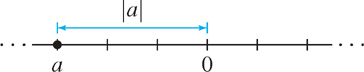
The absolute value of a real number \(a\), denoted \(|a|\), is defined by (Figure 1.2)
\[ |a|=\text{distance from the origin}=\begin{cases} \phantom{-}a&\text{if }a\geq0\\ -a&\text{if }a<0 \end{cases} \]
For example, \(|1.2| = 1.2\) and \(|8.35| = 8.35\). The absolute value satisfies
\[\boxed{|a|=|-a|,\quad|ab|=|a||b|}\]
The distance between two real numbers \(a\) and \(b\) is \(|b - a|\), which is the length of the line segment joining \(a\) and \(b\) (Figure 1.3).
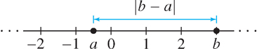
Two real numbers \(a\) and \(b\) are close to each other if \(|b - a|\) is small, and this is the case if their decimal expansions agree to many places. More precisely, if the decimal expansions of \(a\) and \(b\) agree to \(k\) places (to the right of the decimal point), then the distance \( |b - a| \) is at most \(10^{-k}\). Thus, the distance between \(a = 3.1415\) and \(b = 3.1478\) is at most \(10^{-2}\) because \(a\) and \(b\) agree to two places. In fact, the distance is exactly \(|3.1478 - 3.1415| = 0.0063\).
Beware that \(|a + b|\) is not equal to \(|a| + |b|\) unless \(a\) and \(b\) have the same sign or at least one of \(a\) and \(b\) is zero. If they have opposite signs, cancellation occurs in the sum \(a + b\), and \(|a + b| < |a| + |b|\). For example, \(|2 + 5| = |2| + |5|\) but \(|-2 + 5| = 3\), which is less than \(|-2| + |5| = 7\). In any case, \(|a + b|\) is never larger than \(|a| + |b|\) and this gives us the simple but important triangle inequality:
\[ \boxed{|a+b|\leq|a|+|b|}\tag{1} \]
We use standard notation for intervals. Given real numbers \(a \lt b\), there are four intervals with endpoints \(a\) and \(b\) (Figure 1.4). They all have length \(b - a\) but differ according to which endpoints are included.
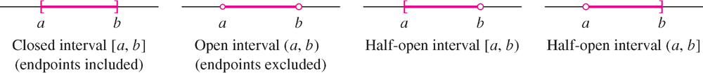
The closed interval \([a, b]\) is the set of all real numbers \(x\) such that \(a \leq x \leq b\):
\[ [a, b] = \{x \in \mathbb{R}: a \leq x \leq b\} \]
We usually write this more simply as \(\{x: a \leq x \leq b\}\), it being understood that \(x\) belongs to \(\mathbb{R}\). The open and half-open intervals are the sets
\[ \underbrace{(a, b) = \{x \in \mathbb{R}: a< x < b\}}_{\text{Open Interval (endpoints excluded)}},\quad \underbrace{[a, b) = \{x \in \mathbb{R}: a\leq x < b\}}_{\text{Half-open Interval}},\quad \underbrace{(a, b] = \{x \in \mathbb{R}: a< x \leq b\}}_{\text{Half-open Interval}} \]
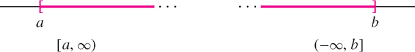
The infinite interval \((-\infty, \infty)\) is the entire real line \(\mathbb{R}\). A half-infinite interval is closed if it contains its finite endpoint and is open otherwise (Figure 1.5):
\[ [a, \infty) = \{x : a \leq x < \infty\}, \quad (-\infty, b] = \{x : -\infty < x \leq b\} \]
3
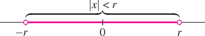
Open and closed intervals may be described by inequalities. For example, the interval \((-r, r)\) is described by the inequality \(|x| \lt r\) (Figure 1.6):
\[ \boxed{|x|<r \Leftrightarrow -r<x<r \Leftrightarrow x\in(-r,r)}\tag{2} \]
More generally, for an interval symmetric about the value \(c\) (Figure 1.7),
\[ \boxed{|x-c|<r \Leftrightarrow c-r<x<c+r \Leftrightarrow x\in (c-r,c+r)}\tag{3} \]
Closed intervals are similar, with \(\lt\) replaced by \(\leq \). We refer to \(r\) as the radius and to \(c\) as the midpoint or center. The intervals\( (a, b)\) and \([a, b]\) have midpoint \(c=\frac{a+b}{2}\) and radius \(r=\frac{b-a}{2}\) (Figure 1.7).
EXAMPLE 1
Describe \([7, 13]\) using inequalities.
Solution The midpoint of the interval \([7, 13]\) is \(c=\frac{1}{2}(7+13)=10\) and its radius is \(r=\frac{1}{2}(13-7)=3\) (Figure 1.8). Therefore,
\[ [7, 13] = \{x \in \mathbb{R} : |x - 10| \leq 3\} \]
EXAMPLE 2
Describe the set \(S =\{x:|\frac{1}{2}x-3|>4\}\) in terms of intervals.
Solution It is easier to consider the opposite inequality \(\frac{1}{2}|x-3|\leq4\) first. By (2),
In Example 2 we use the notation \(\cup\) to denote “union”: The union \(A \cup B\) of sets \(A\) and \(B\) consists of all elements that belong to either \(A\) or \(B\) (or to both).
\begin{align*} \left|\frac{1}{2}x-3\right|\leq4 &\Leftrightarrow -4\leq\frac{1}{2}x-3\leq 4\\ &\Leftrightarrow -1\leq\frac{1}{2}x\leq 7 &&\text{(add 3)}\\ &\Leftrightarrow -2\leq x\leq14 &&\text{(multiply by 2)} \end{align*}
Thus, \(\frac{1}{2}|x-3|\leq4\) is satisfied when \(x\) belongs to \([-2, 14]\). The set \(S\) is the complement, consisting of all numbers \(x\) not in \([-2, 14]\). We can describe \(S\) as the union of two intervals: \(S = (-\infty, -2)\cup (14, \infty)\) (Figure 1.9).
1.1.1 Graphing
The term “Cartesian” refers to the French philosopher and mathematician René Descartes (1596–1650), whose Latin name was Cartesius. He is credited (along with Pierre de Fermat) with the invention of analytic geometry. In his great work La Géométrie, Descartes used the letters \(x, y, z\) for unknowns and \(a, b, c\) for constants, a convention that has been followed ever since.
Graphing is a basic tool in calculus, as it is in algebra and trigonometry. Recall that rectangular (or Cartesian) coordinates in the plane are defined by choosing two perpendicular axes, the \(x\)-axis and the \(y\)-axis. To a pair of numbers \((a, b)\) we associate the point \(P\) located at the intersection of the line perpendicular to the \(x\)-axis at \(a\) and the line perpendicular to the \(y\)-axis at \(b\) [Figure 1.10(A)]. The numbers \(a\) and \(b\) are the \(x\)- and \(y\)-coordinates of P. The \(x\)-coordinate is sometimes called the “abscissa” and the \(y\)-coordinate the “ordinate.” The origin is the point with coordinates \((0, 0)\).
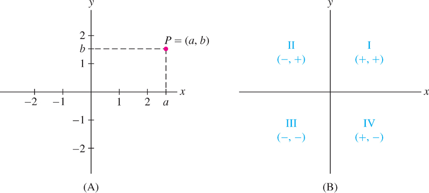
The axes divide the plane into four quadrants labeled I–IV, determined by the signs of the coordinates [Figure 1.10(B)]. For example, quadrant III consists of points \((x, y)\) such that \(x \lt 0\) and\( y \lt 0\).
The distance \(d\) between two points \(P_{1} = (x_{1}, y_{1})\) and \(P_{2} = (x_{2}, y_{2})\) is computed using the Pythagorean Theorem. In Figure 1.11, we see that \(\overline{P_1P_2}\) is the hypotenuse of a right triangle with sides \(a = |x_{2} - x_{1}|\) and \(b = |y_{2} - y_{1}|\). Therefore,
\[ d^{2} = a^{2} + b^{2} = (x_{2} - x_{1})^{2} + (y_{2} - y_{1})^{2} \]
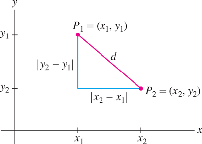
We obtain the distance formula by taking square roots.
4
Distance Formula
Distance Formula The distance between \(P_{1} = (x_{1}, y_{1})\) and \(P_{2} = (x_{2}, y_{2})\) is equal to
\[ \boxed{d=\sqrt{(x_{2} - x_{1})^{2} + (y_{2} - y_{1})^{2}}} \]
Once we have the distance formula, we can derive the equation of a circle of radius \(r\) and center \((a, b)\) (Figure 1.12). A point \((x, y)\) lies on this circle if the distance from \((x, y)\) to \((a, b)\) is \(r\):
\[ \sqrt{(x - a)^{2} + (y - b)^{2}} \]
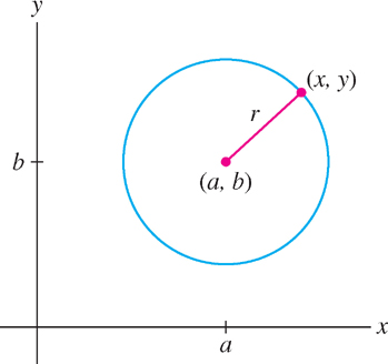
Squaring both sides, we obtain the standard equation of the circle:
\[ \boxed{(x - a)^{2} + (y - b)^{2} = r^{2}} \]
We now review some definitions and notation concerning functions.
DEFINITION
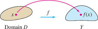
A function \(f\) from a set \(D\) to a set \(Y\) is a rule that assigns, to each element \(x\) in \(D\), a unique element \(y = f (x)\) in \(Y\). We write
\[f : D \rightarrow Y\]
The set \(D\), called the domain of \(f\), is the set of “allowable inputs.” For \(x \in D\), \(f(x)\) is called the value of \(f\) at \(x\) (Figure 1.13). The range \(R\) of \(f\) is the subset of \(Y\) consisting of all values \(f (x)\):
\[ R = \{y \in Y : f (x) = y\text{ for some }x \in D\} \]
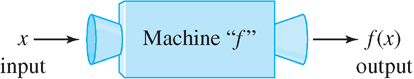
Informally, we think of \(f\) as a “machine” that produces an output \(y\) for every input \(x\) in the domain \(D\) (Figure 1.14).
A function \(f : D \rightarrow Y\) is also called a “map.” The sets \(D\) and \(Y\) can be arbitrary. For example, we can define a map from the set of living people to the set of whole numbers by mapping each person to his or her year of birth. The range of this map is the set of years in which a living person was born. In multivariable calculus, the domain might be a set of points in three-dimensional space and the range a set of numbers, points, or vectors.
5
The first part of this text deals with numerical functions \(f\), where both the domain and the range are sets of real numbers. We refer to such a function interchangeably as \(f\) or \(f(x)\). The letter \(x\) is used often to denote the independent variable that can take on any value in the domain \(D\). We write \(y = f(x)\) and refer to \(y\) as the dependent variable (because its value depends on the choice of \(x\)).
When \(f\) is defined by a formula, its natural domain is the set of real numbers \(x\) for which the formula is meaningful. For example, the function \(f(x)=\sqrt{9-x}\) has domain \(D = \{x : x \leq 9\}\) because \(\sqrt{9-x}\) is defined if \(9 - x \geq 0\). Here are some other examples of domains and ranges:
| \(f (x)\) | Domain \(D\) | Range \(R\) |
|---|---|---|
| \(x^{2}\) | \(\mathbb{R}\) | \(\{y : y \geq 0\}\) |
| \(\cos x\) | \(\mathbb{R}\) | \(\{y : -1 \leq y \leq 1\}\) |
| \(\dfrac{1}{x+1}\) | \(\{x : x \neq -1\}\) | \(\{y : y \neq 0\}\) |
The graph of a function \(y = f (x)\) is obtained by plotting the points \((a, f (a))\) for \(a\) in the domain \(D\) (Figure 1.15). If you start at \(x = a\) on the \(x\)-axis, move up to the graph and then over to the \(y\)-axis, you arrive at the value \(f (a)\). The absolute value \(|f (a)|\) is the distance from the graph to the \(x\)-axis.
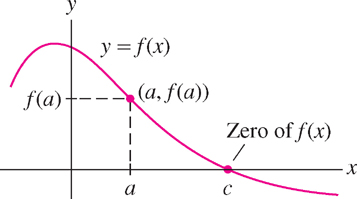
A zero or root of a function \(f (x)\) is a number \(c\) such that \(f (c) = 0\). The zeros are the values of \(x\) where the graph intersects the \(x\)-axis.
In Chapter 4, we will use calculus to sketch and analyze graphs. At this stage, to sketch a graph by hand, we can make a table of function values, plot the corresponding points (including any zeros), and connect them by a smooth curve.
EXAMPLE 3
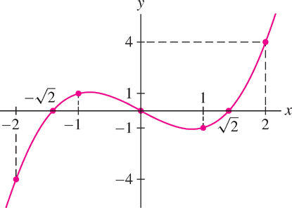
Find the roots and sketch the graph of \(f(x) = x^{3} - 2x\).
Solution First, we solve
\[ x^{3} - 2x = x(x^{2} - 2) = 0. \]
The roots of \(f(x)\) are \(x = 0\) and \(x=\pm\sqrt2\). To sketch the graph, we plot the roots and a few values listed in Table 1.1 and join them by a curve (Figure 1.16).
| \(x\) | \(x^{3} - 2x\) |
|---|---|
| \(-2\) | \(-4\) |
| \(-1\) | \(\phantom{-}1\) |
| \(\phantom{-}0\) | \(\phantom{-}0\) |
| \(\phantom{-}1\) | \(-1\) |
| \(\phantom{-}2\) | \(\phantom{-}4\) |
Functions arising in applications are not always given by formulas. For example, data collected from observation or experiment define functions for which there may be no exact formula. Such functions can be displayed either graphically or by a table of values. Figure 1.17 and Table 1.2 display data collected by biologist Julian Huxley (1887–1975) in a study of the antler weight \(W\) of male red deer as a function of age \(t\). We will see that many of the tools from calculus can be applied to functions constructed from data in this way.
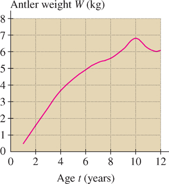
| \(t\) (years) | \(W\) (kg) | \(t\) (years) | \(W\) (kg) |
|---|---|---|---|
| \(1\) | \(0.48\) | \(\phantom{0}7\) | \(5.34\) |
| \(2\) | \(1.59\) | \(\phantom{0}8\) | \(5.62\) |
| \(3\) | \(2.66\) | \(\phantom{0}9\) | \(6.18\) |
| \(4\) | \(3.68\) | \(10\) | \(6.81\) |
| \(5\) | \(4.35\) | \(11\) | \(6.21\) |
| \(6\) | \(4.92\) | \(12\) | \(6.1\phantom{0}\) |
6
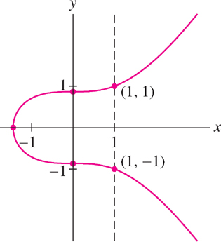
We can graph not just functions but, more generally, plot any equation relating \(y\) and \(x\). Figure 1.18 shows the plot of the equation \(4y^{2} - x^{3} = 3\); it consists of all pairs \((x, y)\) satisfying the equation. This plotted curve is not the graph of a function because some \(x\)-values are associated with two \(y\)-values. For example, \(x = 1\) is associated with \(y = \pm1\). A curve is the graph of a function if and only if it passes the Vertical Line Test; that is, every vertical line \(x = a\) intersects the curve in at most one point.
We are often interested in whether a function is increasing or decreasing. Roughly speaking, a function \(f (x)\) is increasing if its graph goes up as we move to the right and is decreasing if its graph goes down [Figure 1.19(A) and (B)]. More precisely, we define the notion of increase/decrease on an open interval:
- Increasing on \((a, b)\) if \(f(x_{1}) < f(x_{2})\) for all \(x_{1}, x_{2} \in (a, b)\) such that \(x_{1} < x_{2}\)
- Decreasing on \((a, b)\) if \(f(x_{1}) > f(x_{2})\) for all \(x_{1}, x_{2} \in (a, b)\) such that \(x_{1} < x_{2}\)
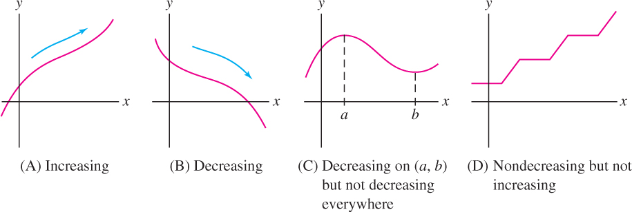
We say that \(f (x)\) is monotonic if it is either increasing or decreasing. In Figure 1.19(C), the function is not monotonic because it is neither increasing nor decreasing for all \(x\).
A function \(f (x)\) is called nondecreasing if \(f (x_{1}) \leq f (x_{2})\) for \(x_{1} < x_{2}\) (defined by \(\leq\) rather than a strict inequality \(<\)). Nonincreasing functions are defined similarly. Function (D) in Figure 19 is nondecreasing, but it is not increasing on the intervals where the graph is horizontal.
Another important property is parity, which refers to whether a function is even or odd:
- \(f (x)\) is even if \(f (-x) = f (x)\)
- \(f (x)\) is odd if \(f (-x) = - f (x)\)
7
The graphs of functions with even or odd parity have a special symmetry:
- Even function: graph is symmetric about the \(y\)-axis. This means that if \(P = (a, b)\) lies on the graph, then so does \(Q = (-a, b)\) [Figure 1.20(A)].
- Odd function: graph is symmetric with respect to the origin. This means that if \(P = (a, b)\) lies on the graph, then so does \(Q = (-a, - b)\) [Figure 1.20(B)].
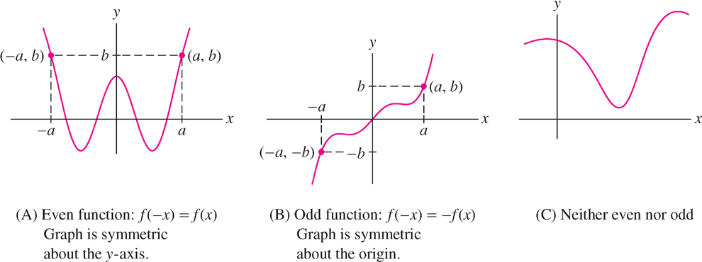
Many functions are neither even nor odd [Figure 1.20(C)].
EXAMPLE 4
Determine whether the function is even, odd, or neither.
(a) \(f(x) = x^{4}\)
(b) \(g(x) = x^{-1}\)
(c) \(h(x) = x^{2} + x\)
Solution
(a) \(f (-x) = (-x)^{4} = x^{4}\). Thus, \(f (x) = f (-x)\) and \(f (x)\) is even.
(b) \(g(-x) = (-x)^{-1} = - x^{-1}\). Thus, \(g(-x) = - g(x)\), and \(g(x)\) is odd.
(c) \(h(-x) = (-x)^{2} + (-x) = x^{2} - x\). We see that \(h(-x)\) is not equal to \(h(x)\) or to \(- h(x) = - x^{2} - x\). Therefore, \(h(x)\) is neither even nor odd.
EXAMPLE 5 Using Symmetry
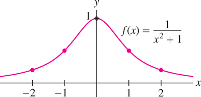
Sketch the graph of \(f(x)=\frac{1}{x^2+1}\).
Solution The function \(f (x)\) is positive \([f (x) \gt 0]\) and even \([f (-x) = f (x)]\). Therefore, the graph lies above the \(x\)-axis and is symmetric with respect to the \(y\)-axis. Furthermore, \(f (x)\) is decreasing for \(x \geq 0\) (because a larger value of \(x\) makes the denominator larger). We use this information and a short table of values (Table 1.3) to sketch the graph (Figure 1.21). Note that the graph approaches the \(x\)-axis as we move to the right or left because \(f (x)\) gets smaller as \(|x|\) increases.
| \(x\) | \(\frac{1}{x^2+1}\) |
| \(\phantom{\pm}0\) | \(1\) |
| \(\pm1\) | \(\frac{1}{2}\) |
| \(\pm2\) | \(\frac{1}{5}\) |
8
Two important ways of modifying a graph are translation (or shifting) and scaling. Translation consists of moving the graph horizontally or vertically:
Remember that \(f (x) + c\) and \(f (x + c) \) are different. The graph of \(y = f (x) + c\) is a vertical translation and \(y = f (x + c) \) a horizontal translation of the graph of \(y = f (x)\).
DEFINITION Translation (Shifting)
- Vertical translation \(y = f (x) + c\): shifts the graph by \(|c|\) units vertically, upward if \(c > 0\) and \(-c\) units downward if \(c < 0\).
- Horizontal translation \(y = f (x + c)\): shifts the graph by \(|c|\) units horizontally, to the right if \(c < 0\) and \(c\) units to the left if \(c > 0\).
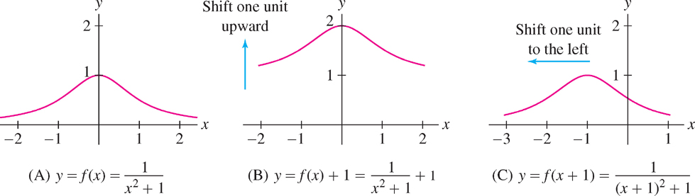
Figure 1.22 shows the effect of translating the graph of \(f (x) = \frac{1}{x^2+1}\) vertically and horizontally.
EXAMPLE 6
Figure 1.23(A) is the graph of \(f (x) = x^{2}\), and Figure 1.23(B) is a horizontal and vertical shift of (A). What is the equation of graph (B)?
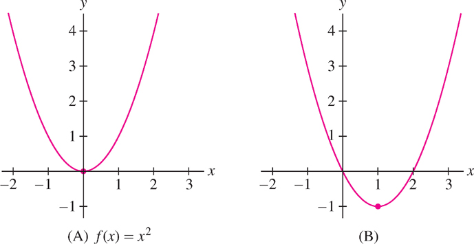
Solution Graph (B) is obtained by shifting graph (A) one unit to the right and one unit down. We can see this by observing that the point \((0, 0)\) on the graph of \(f (x)\) is shifted to \((1, -1)\). Therefore, (B) is the graph of \(g(x) = (x -1)^{2} -1\).
Scaling (also called dilation) consists of compressing or expanding the graph in the vertical or horizontal directions:
DEFINITION Scaling
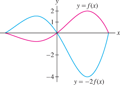
- Vertical scaling \(y = kf (x)\): If \(k \gt 1\), the graph is expanded vertically by the factor \(k\). If \(0 \lt k \lt 1\), the graph is compressed vertically. When the scale factor \(k\) is negative (\(k \lt 0\)), the graph is also reflected across the \(x\)-axis (Figure 1.24).
- Horizontal scaling \(y = f (kx)\): If \(k > 1\), the graph is compressed in the horizontal direction. If \(0 < k < 1\), the graph is expanded. If \(k < 0\), then the graph is also reflected across the \(y\)-axis.
9
We refer to the vertical size of a graph as its amplitude. Thus, vertical scaling changes the amplitude by the factor \(|k|\).
EXAMPLE 7
Remember that \(kf (x)\) and \(f (kx)\) are different. The graph of \(y = kf (x) \) is a vertical scaling, and \(y = f (kx) \) a horizontal scaling, of the graph of \(y = f (x)\).
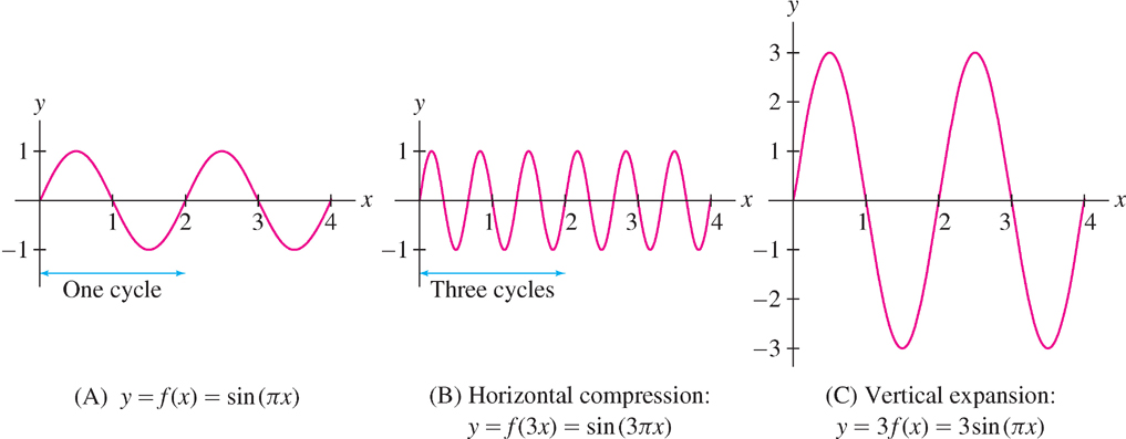
Sketch the graphs of \(f (x) = \sin(\pi x)\) and its dilates \(f (3x)\) and \(3f (x)\).
Solution The graph of \(f (x) = \sin(\pi x) \) is a sine curve with period \(2\). It completes one cycle over every interval of length \(2\) —see Figure 1.25(A).
- The graph of \(f (3x) = \sin(3\pi x)\) is a compressed version of \(y = f (x)\), completing three cycles instead of one over intervals of length \(2\) [Figure 1.25(B)].
- The graph of \(y = 3f (x) = 3 \sin(\pi x)\) differs from \(y = f (x)\) only in amplitude: It is expanded in the vertical direction by a factor of \(3\) [Figure 1.25(C)].
1.1.2 Section 1.1 Summary
- Absolute value: \[ |a|=\begin{cases} \vphantom{-}a&\text{if }a\geq0\\ -a&\text{if }a<0 \end{cases} \]
- Triangle inequality: \(|a + b| \leq |a| + |b|\)
- Four intervals with endpoints a and b:
\[ (a, b),\quad [a, b],\quad [a, b),\quad (a, b] \]
- Writing open and closed intervals using inequalities:
\[ (a, b) = \{x : |x - c| < r\},\quad [a, b] = \{x : |x - c| \leq r\} \]
where \(c=\frac{1}{2}(a+b)\) is the midpoint and \(r=\frac{1}{2}(b-a)\) is the radius.
- Distance \(d\) between \((x_{1}, y_{1})\) and \((x_{2}, y_{2})\):
\[ d=\sqrt{(x_{2} - x_{1})^{2} + (y_{2} - y_{1})^{2}} \]
- Equation of circle of radius \(r\) with center \((a, b)\):
\[ (x - a)^{2} + (y - b)^{2} = r^{2} \]
- A zero or root of a function \(f (x)\) is a number \(c\) such that \(f (c) = 0\).
10
- Vertical Line Test: A curve in the plane is the graph of a function if and only if each vertical line \(x = a\) intersects the curve in at most one point.
Increasing: \(f(x_{1}) < f(x_{2})\) if \(x_{1} < x_{2}\) Nondecreasing: \(f(x_{1}) \leq f(x_{2})\) if \(x_{1} < x_{2}\) Decreasing: \(f(x_{1}) > f(x_{2})\) if \(x_{1} < x_{2}\) Nonincreasing: \(f(x_{1}) \geq f(x_{2})\) if \(x_{1} < x_{2}\)
- Even function: \(f (-x) = f (x)\) (graph is symmetric about the \(y\)-axis).
- Odd function: \(f (-x) = - f (x)\) (graph is symmetric about the origin).
- Four ways to transform the graph of \(f (x)\):
\(f(x) + c\) Shifts graph vertically \(|c|\) units (upward if \(c>0\), downward if \(c < 0\)) \(f(x + c)\) Shifts graph horizontally \(|c|\) units (to the right if \(c < 0\), to the left if \(c > 0\)) \(kf(x)\) Scales graph vertically by factor \(k\); if \(k < 0\), graph is reflected across \(x\)-axis \(f(kx)\) Scales graph horizontally by factor \(k\) (compresses if \(k > 1\)); if \(k < 0\), graph is reflected across \(y\)-axis