1.2 Linear and Quadratic Functions
Linear functions are the simplest of all functions, and their graphs (lines) are the simplest of all curves. However, linear functions and lines play an enormously important role in calculus. For this reason, you should be thoroughly familiar with the basic properties of linear functions and the different ways of writing an equation of a line.
Let’s recall that a linear function is a function of the form
\[ \boxed{f(x)=mx+b\quad\text{(\(m\) and \(b\) constants)}} \]
The graph of \(f(x)\) is a line of slope \(m\), and since \(f(0) = b,\) the graph intersects the \(y\)-axis at the point \((0, b)\) (Figure 1.26). The number \(b\) is called the \(y\)-intercept, and the equation \(y = mx + b\) for the line is said to be in slope-intercept form.
We use the symbols \(\Delta x\) and \(\Delta y\) to denote the change (or increment) in \(x\) and \(y = f(x)\) over an interval \([x_{1}, x_{2}]\) (Figure 1.26):
\[ \Delta x=x_2-x_1,\quad\Delta y = y_2-y_1 = f(x_2)-f(x_1) \]
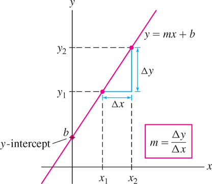
The slope \(m\) of a line is equal to the ratio
\[ m=\frac{\Delta y}{\Delta y} = \frac{\text{vertical change}}{\text{horizontal change}}=\frac{\text{rise}}{\text{run}} \]
This follows from the formula \(y = mx + b\):
\[ \frac{\Delta y}{\Delta x}= \frac{y_2-y_1}{x_2-x_1} = \frac{(mx_1+b) - (mx_2+b)}{x_2 - x_1}= \frac{m(x_2-x_1)}{x_2-x_1}=m \]
14
The slope \(m\) measures the rate of change of \(y\) with respect to \(x\). In fact, by writing
\[ \Delta y = m\Delta x \]
we see that a one-unit increase in \(x\) (i.e., \(\Delta x = 1\)) produces an \(m\) -unit change \(\Delta y\) in \(y\). For example, if \(m = 5\), then \(y\) increases by five units per unit increase in \(x\). The rate-of-change interpretation of the slope is fundamental in calculus. We discuss it in greater detail in Section 2.1.
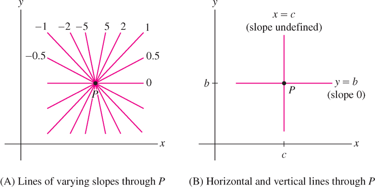
Graphically, the slope \(m\) measures the steepness of the line \(y = mx + b\). Figure 1.27(A) shows lines through a point of varying slope \(m\). Note the following properties:
- Steepness: The larger the absolute value \(|m|\), the steeper the line.
- Negative slope: If \(m < 0\), the line slants downward from left to right.
- \(f(x) = mx + b\) is increasing if \(m > 0\) and decreasing if \(m < 0\).
- The horizontal line \(y = b\) has slope \(m = 0\) [Figure 1.27(B)].
- A vertical line has equation \(x = c\), where \(c\) is a constant. The slope of a vertical line is undefined. It is not possible to write the equation of a vertical line in slope-intercept form \(y = mx + b\).
CAUTION:
Graphs are often plotted using different scales for the \(x\)-and \(y\)-axes. This is necessary to keep the sizes of graphs within reasonable bounds. However, when the scales are different, lines do not appear with their true slopes.
Scale is especially important in applications because the steepness of a graph depends on the choice of units for the \(x\)- and \(y\)-axes. We can create very different subjective impressions by changing the scale. Figure 1.28 shows the growth of company profits over a four-year period. The two plots convey the same information, but the upper plot makes the growth look more dramatic.

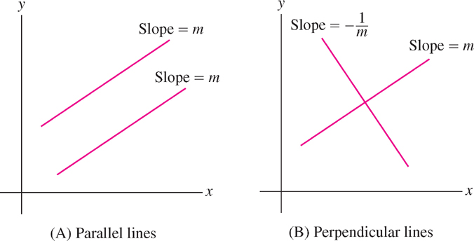
Next, we recall the relation between the slopes of parallel and perpendicular lines (Figure 1.29):
- Lines of slopes \(m_{1}\) and \(m_{2}\) are parallel if and only if \(m_{1} = m_{2}\).
- Lines of slopes m1 and m2 are perpendicular if and only if
\[ m_1 = -\frac{1}{m_2}\quad\text{(or \(m_1m_2=-1\))} \]
15
CONCEPTUAL INSIGHT
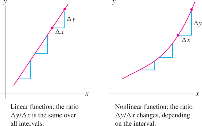
The increments over an interval \([x_{1}, x_{2}]\):
\[ \Delta x = x_{2} - x_{1},\quad \Delta y = f(x_{2}) - f(x_{1}) \]
are defined for any function \(f(x)\) (linear or not), but the ratio \(\frac{\Delta y}{\Delta x}\) may depend on the interval (Figure 1.30). The characteristic property of a linear function \(f(x) = mx + b\) is that \(\frac{\Delta y}{\Delta x}\) has the same value \(m\) for every interval. In other words, \(y\) has a constant rate of change with respect to \(x\). We can use this property to test if two quantities are related by a linear equation.
EXAMPLE 1 Testing for a Linear Relationship
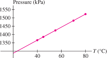
Do the data in Table 1.4 suggest a linear relation between the pressure \(P\) and temperature \(T\) of a gas?
| Temperature (°C) | Pressure (kPa) |
|---|---|
| 40 | 1365.80 |
| 45 | 1385.40 |
| 55 | 1424.60 |
| 70 | 1483.40 |
| 80 | 1522.60 |
16
Real experimental data are unlikely to reveal perfect linearity, even if the data points do essentially lie on a line. The method of “linear regression” is used to find the linear function that best fits the data.
Solution We calculate \(\frac{\Delta P}{\Delta T}\) at successive data points and check whether this ratio is constant:
\[ \begin{array}{ccc} \hline (T_1,P_1)&(T_2,P_2)&\dfrac{\Delta P}{\Delta T}\\[5pt] \hline (40, 1365.80)&(45,1385.40)&\dfrac{1385.40 - 1365.80}{45-40}=3.92\\[5pt] (45,1385.40)&(55,1424.60)&\dfrac{1424.60-1385.40}{55-45}=3.92\\[5pt] (55,1424.60)&(70,1483.40)&\dfrac{1483.40-1424.60}{70-55}=3.92\\[5pt] (70,1483.40)&(80,1522.60)&\dfrac{1522.60-1483.40}{80-70}=3.92\\[5pt] \hline \end{array} \]
Because \(\frac{\Delta P}{\Delta T}\) has the constant value \(3.92\), the data points lie on a line with slope \(m = 3.92\) (this is confirmed in the plot in Figure 1.31).
As mentioned above, it is important to be familiar with the standard ways of writing the equation of a line. The general linear equation is
\[ \boxed{ax+by=c}\tag{1} \]
where \(a\) and \(b\) are not both zero. For \(b = 0\), we obtain the vertical line \(ax = c\). When \(b \neq 0\), we can rewrite Eq. (1) in slope-intercept form. For example, \(-6x + 2y = 3\) can be rewritten as \(y=3x+\frac{3}{2}\).
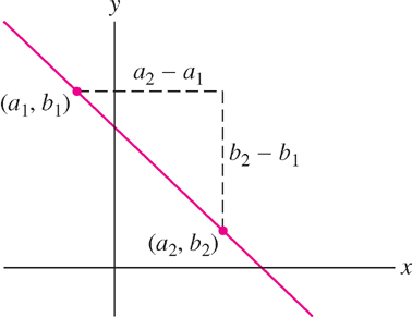
Two other forms we will use frequently are the point-slope and point-point forms. Given a point \(P = (a, b)\) and a slope \(m\), the equation of the line through \(P\) with slope \(m\) is \(y - b = m(x - a)\). Similarly, the line through two distinct points \(P = (a_{1}, b_{1}) and Q = (a_{2}, b_{2})\) has slope (Figure 1.32)
\[ m=\frac{b_2-b_1}{a_2-a_1} \]
Therefore, we can write its equation as \(y - b_{1} = m(x - a_{1})\).
Equations for Lines
- 1. Point-slope form of the line through \(P = (a, b)\) with slope \(m\):
\[ \boxed{y-b=m(x-a)} \]
- 2. Point-point form of the line through \(P = (a_{1}, b_{1})\) and \(Q = (a_{2}, b_{2})\):
\[ y-b_1 = m(x-a_1)\quad\text{where } m=\frac{b_2-b_1}{a_2-a_1} \]
17
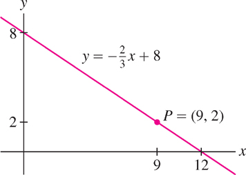
EXAMPLE 2 Line of Given Slope Through a Given Point
Find the equation of the line through \((9, 2)\) with slope \(-\frac{2}{3}\).
Solution In point-slope form:
\[ y-2 = -\frac{2}{3}(x-9) \]
In slope-intercept form: \(y=-\frac{2}{3}(x-9)+2\) or \(y=-\frac{2}{3}x+8\). See Figure 1.33.
EXAMPLE 3 Line Through Two Points
Find the equation of the line through \((2, 1)\) and \((9, 5)\).
Solution The line has slope
\[ m = \frac{5-1}{9-2}=\frac{4}{7} \]
Because \((2, 1)\) lies on the line, its equation in point-slope form is \(y-1=\frac{4}{7}(x-2)\).
A quadratic function is a function defined by a quadratic polynomial
\[ f(x) = ax^{2} + bx + c \quad(a, b, c\text{ constants with }a \neq 0) \]
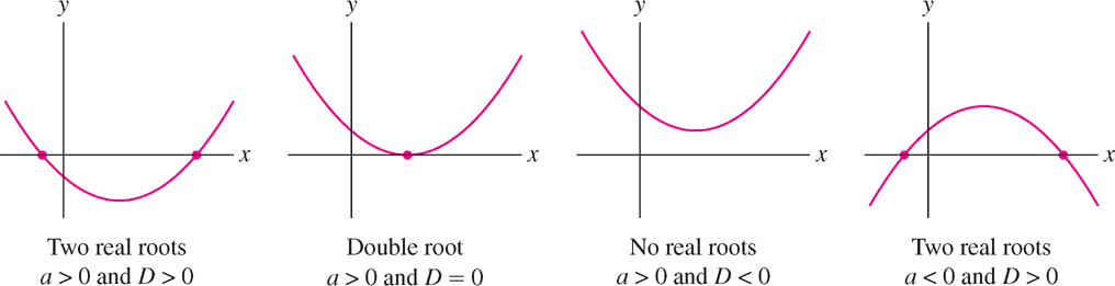
The graph of \(f(x)\) is a parabola (Figure 1.34). The parabola opens upward if the leading coefficient \(a\) is positive and downward if \(a\) is negative. The discriminant of \(f(x)\) is the quantity
\[ D = b^{2} - 4ac \]
The roots of \(f(x)\) are given by the quadratic formula (see Exercise 56):
\[ \text{Roots of }f(x) = \frac{-b\pm\sqrt{b^2-4ac}}{2}=\frac{-b\pm\sqrt D}{2a} \]
The sign of \(D\) determines whether or not \(f(x)\) has real roots (Figure 1.34). If \(D \gt 0\), then \(f(x)\) has two real roots, and if \(D = 0\), it has one real root (a “double root”). If \(D \lt 0\), then \(\sqrt{D}\) is imaginary and \(f(x)\) has no real roots.
When \(f(x)\) has two real roots \(r_{1}\) and \(r_{2}\), then \(f(x)\) factors as
\[ f(x) = a(x - r_{1})(x - r_{2}) \]
For example, \(f(x) = 2x^{2} - 3x + 1\) has discriminant \(D = b^{2} - 4ac = 9 - 8 = 1 > 0\), and by the quadratic formula, its roots are \(\frac{3\pm1}{4}\) or \(1\) and \(\frac{1}{2}\). Therefore,
\[ f(x) = 2x^2 - 3x + 1 =2(x-1)\left(x-\frac{1}{2}\right) \]
18
The technique of completing the square consists of writing a quadratic polynomial as a multiple of a square plus a constant:
\[ \boxed{ax^2 + bx + c = a \underbrace{\left(x+\dfrac{b}{2a}\right)^2}_{\text{Square term}} + \underbrace{\dfrac{4ac-b^2}{4a}}_{\text{Constant}}}\tag{2} \]
It is not necessary to memorize this formula, but you should know how to carry out the process of completing the square.
EXAMPLE 4 Completing the Square
Cuneiform texts written on clay tablets show that the method of completing the square was known to ancient Babylonian mathematicians who lived some 4000 years ago.
Complete the square for the quadratic polynomial \(4x^{2} - 12x + 3\).
Solution First factor out the leading coefficient:
\[ 4x^2 - 12x + 3 = 4 \left(x^2-3x+\frac{3}{4}\right) \]
Then complete the square for the term \(x^{2} - 3x\):
\[ x^2 + bx = \left(x + \frac{b}{2}\right)^2 - \frac{b^2}{4}, \quad x^2 - 3x = \left(x - \frac{3}{2}\right)^2 - \frac{9}{4} \]
Therefore,
\[ 4x^2 - 12x + 3 = 4 \left(\left(x - \frac{3}{2}\right)^2 - \frac{9}{4} + \frac{3}{4}\right) = 4 \left(x - \frac{3}{2}\right)^2 - 6 \]
The method of completing the square can be used to find the minimum or maximum value of a quadratic function.
EXAMPLE 5 Finding the Minimum of a Quadratic Function
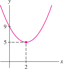
Complete the square and find the minimum value of \(f(x) = x^{2} - 4x + 9\).
Solution We have
\[ f(x) = x^2 - 4x + 9 = (x-2)^2 - 4 + 9 = \overbrace{(x-2)^2}^{\text{This term is }\geq 0}+5 \]
Thus, \(f(x) \geq 5\) for all \(x\), and the minimum value of \(f(x)\) is \(f(2) = 5\) (Figure 1.35).
1.2.1 Section 1.2 Summary
- A linear function is a function of the form \(f(x) = mx + b\).
- The general equation of a line is \(ax + by = c\). The line \(y = c\) is horizontal and \(x = c\) is vertical.
- Three convenient ways of writing the equation of a nonvertical line:
- – Slope-intercept form: \(y = mx + b\) (slope \(m\) and \(y\)-intercept \(b\))
- – Point-slope form: \(y - b = m(x - a)\) [slope \(m,\) passes through \((a, b)\)]
- – Point-point form: The line through two points \(P = (a_{1}, b_{1})\) and \(Q = (a_{2}, b_{2})\) has slope \(m=\frac{b_2-b_1}{a_2-a_1}\) and equation \(y - b_{1} = m(x - a_{1})\).
- Two lines of slopes \(m_{1}\) and \(m_{2}\) are parallel if and only if \(m_{1} = m_{2}\), and they are perpendicular if and only if \(m_{1} = -\frac{1}{m_2}\).
- Quadratic function: \(f(x) = ax^{2} + bx + c\). The roots are \(m=\frac{-b\pm\sqrt{D}}{2a}\), where \(D = b^{2} - 4ac\) is the discriminant. The roots are real and distinct if \(D > 0\), there is a double root if \(D = 0\), and there are no real roots if \(D < 0\).
- Completing the square consists of writing a quadratic function as a multiple of a square plus a constant.
19