2.2 Limits: A Numerical and Graphical Approach
In the last section we considered the instantaneous rate of change as the limiting value of \(\frac{\Delta s}{\Delta t}\)as \(\Delta t\) tends to zero (we write \(\Delta t \rightarrow 0\)). We denote this limiting value (assuming it exists) as \[\lim_{\Delta t \rightarrow 0} \frac{\Delta s}{\Delta t}\]
To understand the idea of a limiting value more deeply (the central idea that lies at the very heart of calculus), we should make a transition and consider a general function \(f\) of a variable (say \(x\); so \(y=f(x)\)) and ask the question: what happens to \(f(x)\) as \(x\) goes to some number \(c\) (\(x \rightarrow c\)). This is a generalization of the question of what happens to \(\frac{\Delta s}{\Delta t} =: f(\Delta t)\) (we consider here \(\frac{\Delta s}{\Delta t}\) as a function of \(\Delta t\)) as \(\Delta t \rightarrow 0\). In that setting we are varying \(\Delta t\) and letting \(\Delta t \rightarrow 0\) and now we are varying \(x\) and letting \(x \rightarrow c\).
Thus, the goal in this section is to define limits and study them using numerical, graphical and algebraic techniques. We begin with the following question: How do the values of a function \(f(x)\) behave when \(x\) approaches a number \(c\), whether or not \(f(x)\) is defined?
2.2.1 Definition of a Limit
To define limits, let us recall that the distance between two numbers \(a\) and \(b\) is the absolute value \(|a-b|\), so we can express the idea that \(f(x)\) is close to \(L\) by saying that \(|f(x) − L|\) is small.
50
The limit concept was not fully clarified until the nineteenth century. The French mathematician Augustin-Louis Cauchy (1789–1857, pronounced Koh-shee) gave the following verbal definition: “When the values successively attributed to the same variable approach a fixed value indefinitely, in such a way as to end up differing from it by as little as one could wish, this last value is called the limit of all the others. So, for example, an irrational number is the limit of the various fractions which provide values that approximate it more and more closely.” (Translated by J. Grabiner)
The first mathematically precise definition is due to the German mathematician Karl Weierstraß (1815-1897), given in his Berlin lectures.
DEFINITION Limit
Assume that \(f(x)\) is defined for all \(x\) in an open interval containing \(c\), but not necessarily at \(c\) itself. We say that
the limit of \(f(x)\) as \(x\) approaches \(c\) is equal to \(L\)
if \(|f(x) − L|\) becomes arbitrarily small when \(x\) is any number sufficiently close (but not equal) to \(c\). In this case, we write \[\lim\limits_{x\rightarrow c} f(x) = L\]
We also say that \(f(x)\) approaches or converges to \(L\) as \(x\rightarrow c\) (and we write \(f(x) \rightarrow L\)).
If the values of \(f(x)\) do not converge to any limit as \(x\rightarrow c\), we say that \(\lim\limits_{x\rightarrow c}f(x)\) does not exist. It is important to note that the value \(f(c)\) itself, which may or may not be defined, plays no role in the limit. All that matters are the values of \(f(x)\) for \(x\) close to \(c\). Furthermore, if \(f(x)\) approaches a limit as \(x\rightarrow c\), then the limiting value \(L\) is unique.
EXAMPLE 1
Use the definition above to verify the following limits:
(a) \(\displaystyle \lim \limits_{x \rightarrow 7} 5=5\)
(b) \(\displaystyle \lim \limits_{x \rightarrow 4} (3x+1)=13\)
Solution
(a) Let \(f(x)=5\). To show that \(\displaystyle \lim \limits_{x \rightarrow 7} 5=5\), we must show that \(|f(x) - 5|\) becomes arbitrarily small when \(x\) is sufficiently close (but not equal) to 7. But observe that \(|f(x) - 5| = |5-5| = 0\) for all \(x\), so what we are required to show is automatic (and it is not necessary to take \(x\) close to 7).
(b) Let \(f(x) = 3x+1\). To show that \(\displaystyle \lim \limits_{x \rightarrow 4} 3x+1=13\), we must show that \(|f(x) – 13|\) becomes arbitrarily small when \(x\) is sufficiently close (but not equal) to 4. We have \[|f(x) - 13| = |(3x+1) - 13| = |3x - 12| = 3|x-4|\] Because \(|f(x) – 13|\) is a multiple of \(|x– 4|\), we can make \(|f(x) – 13|\) arbitrarily small by taking \(x\) sufficiently close to 4.
Reasoning as in Example 1 but with arbitrary constants, we obtain the following simple but important results:
THEOREM 1
For any constants \(k\) and \(c\), (a) \(\displaystyle \lim \limits_{x \rightarrow c} k=k\) and (b) \(\displaystyle \lim \limits_{x \rightarrow c} x=c\).
Question 2.5 Limit Progress Check Question 1
| \(\lim \limits_{x \rightarrow 5} 3 = \) | 607M7xmPORU= |
|---|---|
| \(\lim \limits_{x \rightarrow 5} x = \) | DYU2tVvtzEQ= |
To deal with more complicated limits and especially, to provide mathematically rigorous proofs, a more precise version of the above limit definition is needed. This more precise version is discussed in Section 2.9, where inequalities are used to pin down the exact meaning of the phrases “arbitrarily small” and “sufficiently close.”
2.2.2 Graphical and Numerical Investigation
Graphical and numerical investigations provide evidence for a limit, but they do not prove that the limit exists or has a given value. This is done for instance by using the Limit Laws or other theorems established in the following sections.
Our goal in the rest of this section is to develop a better intuitive understanding of limits by investigating them graphically and numerically.
Graphical Investigation Use a graphing utility to produce a graph of \(f(x)\). The graph should give a visual impression of whether or not a limit exists. It can often be used to estimate the value of the limit.
51
Numerical Investigation We write \(x\rightarrow c^-\) to indicate that \(x\) approaches \(c\) through values less than \(c\), and we write \(x\rightarrow c^+\) to indicate that \(x\) approaches \(c\) through values greater than \(c\). To investigate \(\lim\limits_{x\rightarrow c} f(x)\),
- (i) Make a table of values of \(f(x)\) for \(x\) close to but less than \(c\) —that is, as \(x\rightarrow c^-\).
- (ii) Make a second table of values of \(f(x)\) for \(x\) close to but greater than \(c\) —that is, as \(x\rightarrow c^+\).
- (iii) If both tables indicate convergence to the same number \(L\), we take \(L\) to be an estimate for the limit.
The tables should contain enough values to reveal a clear trend of convergence to a value \(L\). If \(f(x)\) approaches a limit, the successive values of \(f(x)\) will generally agree to more and more decimal places as \(x\) is taken closer to \(c\). If no pattern emerges, then the limit may not exist.
The undefined expression \(\tfrac{0}{0}\) is referred to as an “indeterminate form.”
EXAMPLE 1
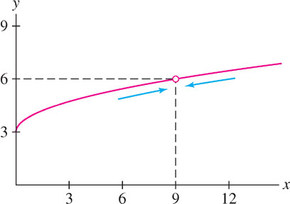
Investigate \(\lim\limits_{x\rightarrow 9}\frac{x-9}{\sqrt{x}-3}\) graphically and numerically.
Solution The function \(f(x) = \frac{x-9}{\sqrt{x}-3}\) is undefined at \(x=9\) because the formula for \(f(9)\) leads to the undefined expression \(\tfrac{0}{0}\). Therefore, the graph in Figure 2.9 has a gap at \(x=9\). However, the graph suggests that \(f(x)\) approaches 6 as \(x\rightarrow 9\).
For numerical evidence, we consider a table of values of \(f(x)\) for \(x\) approaching 9 from both the left and the right. Table 2.4 confirms our impression that \[\lim\limits_{x\rightarrow 9}\frac{x-9}{\sqrt{x}-3} = 6\]
| \(x\rightarrow 9^-\) | \(\frac{x-9}{\sqrt{x}-3}\) | \(x\rightarrow 9^+\) | \(\frac{x-9}{\sqrt{x}-3}\) |
|---|---|---|---|
| 8.9 | 5.98329 | 9.1 | 6.01662 |
| 8.99 | 5.99833 | 9.01 | 6.001666 |
| 8.999 | 5.99983 | 9.001 | 6.000167 |
| 8.9999 | 5.9999833 | 9.0001 | 6.0000167 |
EXAMPLE 2 Limit Equals Function Value
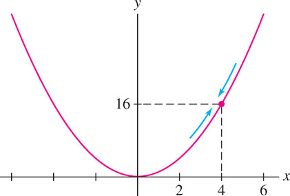
Investigate \(\lim\limits_{x\rightarrow 4} x^2\).
SolutionFigure 2.10 and Table 2.5 both suggest that \(\lim\limits_{x\rightarrow 4} x^2 = 16\). But \(f(x) = x^2\) is defined at \(x=4\) and \(f(4)=16\), so in this case, the limit is equal to the function value. This pleasant conclusion is valid whenever \(f(x)\) is a continuous function, a concept treated in Section 2.2.5.
52
| \(x\rightarrow 4^-\) | \(x^2\) | \(x\rightarrow 4^+\) | \(x^2\) |
|---|---|---|---|
| 3.9 | 15.21 | 4.1 | 16.81 |
| 3.99 | 15.9201 | 4.01 | 16.0801 |
| 3.999 | 15.992001 | 4.001 | 16.008001 |
| 3.9999 | 15.99920001 | 4.0001 | 16.00080001 |
The following example illustrates why in some cases we can use algebraic methods to calculate the limit.
EXAMPLE 3
Reinvestigate \(\lim\limits_{x\rightarrow 9}\dfrac{x-9}{\sqrt{x}-3}\) algebraically.
Solution We will algebraically rewrite the expression using a technique called "rationalizing the denominator" to obtain clear solid evidence as to why the guess for the value of the limit in example one above is correct: \[\lim\limits_{x\rightarrow 9}\frac{x-9}{\sqrt{x}-3} = \lim\limits_{x\rightarrow 9}\frac{x-9}{\sqrt{x}-3} \cdot \frac{\sqrt{x}+3}{\sqrt{x}+3} = \lim\limits_{x\rightarrow 9}\frac{{(x-9)}(\sqrt{x}+3)}{{(x-9)}\cdot 1} = \lim\limits_{x\rightarrow 9} \sqrt{x} + 3\]
As in example two, we can evaluate the last limit by finding the function value of \(g(x) = \sqrt{x} + 3\) when \(x=9\), which evaluates to 6. Note that this was not possible before since this would have required us to divide by zero. The purpose of the algebraic rewrite was to eliminate this problem. Why this is justified in this case will be discussed in the next sections.
Question 2.6 Limit Progress Check Question 2
rZNaBgFCCEop0LeasVY2sbbNJKIqenMKWK9BXt39CWYPgUKyUQeImrVM+V7GCBq/PnKojQREjNhOZ45xMJBZGnEbgFfK4dZ1EXAMPLE 4
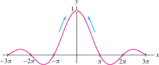
Investigate \(\lim\limits_{x\rightarrow 0} \dfrac{\sin x}{x}\) graphically and numerically.
49
To investigate this limit, consider the graph of \(f(x) = \frac{\sin x}{x}\) given in Figure 2.11. The graph gives the unmistakable impression that \(f(x)\) gets closer and closer to 1 as \(x\rightarrow 0^+\) and as \(x\rightarrow 0^-\).
This conclusion is supported by the table of values for \(f(x)\) for \(x\) near 0 in Table 2.6. Therefore both the graphical and numerical evidence suggest that \(\lim\limits_{x\rightarrow 0} \frac{\sin x}{x} = 1\).
| \(x\) | \(\frac{\sin x}{x}\) | \(x\) | \(\frac{\sin x}{x}\) |
|---|---|---|---|
| 1 | 0.841470985 | −1 | 0.841470985 |
| 0.5 | 0.958851077 | −0.5 | 0.958851077 |
| 0.1 | 0.998334166 | −0.1 | 0.998334166 |
| 0.05 | 0.999583385 | −0.05 | 0.999583385 |
| 0.01 | 0.999983333 | −0.01 | 0.999983333 |
| 0.005 | 0.999995833 | −0.005 | 0.999995833 |
| 0.001 | 0.999999833 | −0.001 | 0.999999833 |
| \(x\rightarrow 0^+\) | \(f(x)\rightarrow 1\) | \(x\rightarrow 0^-\) | \(f(x)\rightarrow 1\) |
CAUTION Numerical investigations are often suggestive, but may be misleading in some cases. If, in Example 5, we had chosen to evaluate \(f(x) = \sin\frac{\pi}{x}\) at the values \(x = 0.1, 0.01, 0.001,\ldots\) we might have concluded incorrectly that \(f(x)\) approaches the limit \(0\) as \(x\rightarrow 0\). The problem is that \(f(10^{-n}) = \sin(10^n\pi) = 0\) for every whole number \(n\), but \(f(x)\) itself does not approach any limit.
EXAMPLE 5 A Limit That Does Not Exist
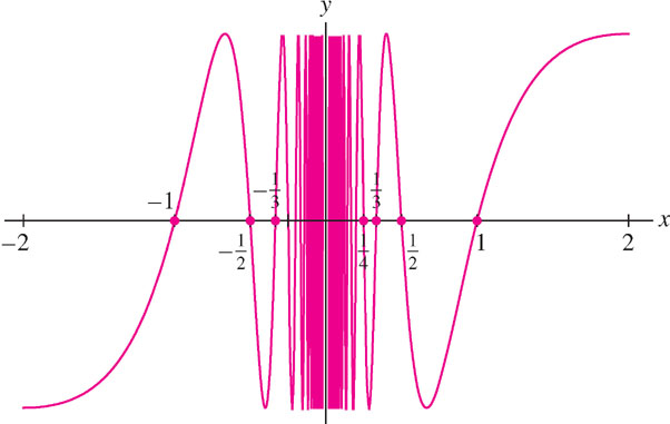
Investigate \(\lim\limits_{x\rightarrow 0} \sin\frac{\pi}{x}\) graphically and numerically.
Solution The function \(f(x) = \sin\frac{\pi}{x}\) is not defined at \(x=0\), but Figure 2.12 suggests that it oscillates between +1 and −1 infinitely often as \(x\rightarrow 0\). It appears, therefore, that \(\lim\limits_{x\rightarrow 0} \sin\frac{\pi}{x}\) does not exist. This impression is confirmed by Table 2.7, which shows that the values of \(f(x)\) bounce around and do not tend toward any limit \(L\) as \(x\rightarrow 0\).
| \(x\rightarrow 0^-\) | \(\sin\frac{\pi}{x}\) | \(x\rightarrow 0^+\) | \(\sin\frac{\pi}{x}\) |
|---|---|---|---|
| −0.1 | 0 | 0.1 | 0 |
| −0.03 | 0.866 | 0.03 | −0.866 |
| −0.007 | −0.434 | 0.007 | 0.434 |
| −0.0009 | 0.342 | 0.0009 | −0.342 |
| −0.00065 | −0.935 | 0.00065 | 0.935 |
53
2.2.3 One-Sided Limits
The limits discussed so far are two-sided. To show that \(\lim\limits_{x\rightarrow c} f(x) = L\), it is necessary to check that \(f(x)\) converges to \(L\) as \(x\) approaches \(c\) through values both larger and smaller than \(c\). In some instances, \(f(x)\) may approach \(L\) from one side of \(c\) without necessarily approaching it from the other side, or \(f(x)\) may be defined on only one side of \(c\). For this reason, we define the one-sided limits \[\lim\limits_{x\rightarrow c^-} f(x) \text{ (left-hand limit)},\quad \lim\limits_{x\rightarrow c^+} f(x) \text{ (right-hand limit)}\]
We now have
THEOREM 1
The limit itself exists if and only if both one-sided limits exist and are equal.
The proof of this theorem is straightforward but requires a more formal definition of limit. It is presented as a video in Section 2.9.
EXAMPLE 6 Left- and Right-Hand Limits Not Equal
Investigate the one-sided limits of \(f(x) = \frac{x}{|x|}\) as \(x\rightarrow 0\). Does \(\lim\limits_{x\rightarrow 0} f(x)\) exist?
Solution For \(x < 0\), \[f(x) = \frac{x}{|x|} = \frac{x}{-x} = -1\]
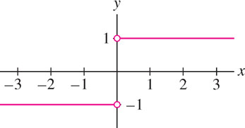
Therefore, the left-hand limit is \(\lim\limits_{x\rightarrow 0^-} f(x) = -1\). But for \(x > 0\), \[f(x) = \frac{x}{|x|} = \frac{x}{x} = 1\]
Therefore, \(\lim\limits_{x\rightarrow 0^+} f(x) = 1\). These one-sided limits are not equal, so \(\lim\limits_{x\rightarrow 0} f(x)\) does not exist.
Question 2.7 Limit Progress Check Question 3
aoMSj1uPr8QsfA2i3VKUmST607BQfZrfmS6tvXBoryhL3PqYtNlrlnjCUnm6JoRr5WhKZnFJi33zIEOWFLknCsPTSEePCYy8IfK+N3pOoHwaf5XAu9ulC6OHbJTLLdkathhO2fNzYqp7nwH7uAXpTGOLpJM72rh9BdE6UmIL5WNbVKtGBz3ibX9NzrydmgSauf4n6FHsdDPi/pSzoeoN8rF4J3sKqu5PZZuvq4Dpc4faSXMXfx/l7+JT00h9Gsv2X2YpQny1oxIeeGi3n8kxneirJYX7Wtjzr2BBsR5/uRG+u190nUL1qiPKnboX0I1guSPKSIT/NFJKe735tATm1RTHqsRjUSPS64DRhOMMid5qQKt+p9aVBe/e/X2KFDec/KMQHhXcEmzjvbGLqhWFOALT2OGR2a4/g1LgsgzEyPVBvcMiD0besVZiDdIPr0pxVEIoZlCscY9HbUGkvHHP79xo/tebWrlaxJ6XAogDn216HEr+kl6Uw9yW8dTlsNfZFXV1bU6zud1mpKXAC6Nd1M8E0W83ayYxtGr7I3ZiJKyfz5sefOFZ+Q==EXAMPLE 7
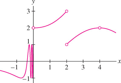
The function \(f(x)\) in Figure 2.14 is not defined at \(c = 0, 2, 4\). Investigate the one- and two-sided limits at these points.
Solution
- \(c=0\): The left-hand limit \(\lim\limits_{x\rightarrow 0^-} f(x)\) does not seem to exist because \(f(x)\) appears to oscillate infinitely often to the left of \(x=0\). On the other hand, \(\lim\limits_{x\rightarrow 0^+} f(x) = 2\).
- \(c=2\): The one-sided limits exist but are not equal: \(\lim\limits_{x\rightarrow 2^-} f(x) = 3\) and \(\lim\limits_{x\rightarrow 2^+} f(x) = 1\). Therefore, \(\lim\limits_{x\rightarrow 2} f(x)\) does not exist.
- \(c=4\): The one-sided limits exist and both have the value 2. Therefore, the two-sided limit exists and \(\lim\limits_{x\rightarrow 4} f(x) = 2\).
Example 8
The applet below lets you visualize that, as \(x \rightarrow 2\), \(f(x)\) approaches a different value from the left as from the right. Thus, the one-sided limits are not equal, and \(\lim\limits_{x \rightarrow 2} f(x)\) does not exist.

2.2.4 Infinite Limits
CAUTION To write that \(\lim\limits_{x\rightarrow c}f(x)=\infty\) is really an abuse of notation since in reality \(\lim\limits_{x\rightarrow c}f(x)\) does not exist in this case. However, stating that \(\lim\limits_{x\rightarrow c}f(x) = \infty\) conveys the information that \(f(x)\) becomes larger and larger as \(x\) gets closer and closer to \(c\). This is useful information about the behavior of the function \(y=f(x)\) near \(x=c\) and therefore we allow this abuse of notation.
Some functions \(f(x)\) tend to \(\infty\) or \(-\infty\) as \(x\) approaches a value \(c\). If so, \(\lim\limits_{x\rightarrow c}f(x)\) does not exist, but we say that \(f(x)\) has an infinite limit. More precisely, we write
- \(\lim\limits_{x\rightarrow c}f(x) = \infty\) if \(f(x)\) increases without bound as \(x\rightarrow c\).
- \(\lim\limits_{x\rightarrow c}f(x) = -\infty\) if \(f(x)\) decreases without bound as \(x\rightarrow c\).
Here, “decrease without bound” means that \(f(x)\) becomes negative and \(|f(x)|\rightarrow\infty\). One-sided infinite limits are defined similarly. When using this notation, keep in mind that \(\infty\) and \(-\infty\) are not real numbers.
When \(f(x)\) approaches \(\infty\) or \(-\infty\) as as \(x\) approaches \(c\) from one or both sides, the line \(x=c\) is called a vertical asymptote. For example, as you can see in the figures below, the line \(x=0\) is a vertical asymptote for both functions in Example 8 as well in Examples 9(b) and 9(c). In Example 9(a), the line \(x=2\) is the vertical asymptote.
Example 8
54
In the next example, the notation \(x\rightarrow c^\pm\) is used to indicate that the left- and right-hand limits are to be considered separately.
EXAMPLE 9
Investigate the one-sided limits graphically:
(a) \(\lim\limits_{x\rightarrow 2^\pm}\dfrac{1}{x-2}\)
(b) \(\lim\limits_{x\rightarrow 0^\pm}\dfrac{1}{x^2}\)
(c) \(\lim\limits_{x\rightarrow 0^+}\ln(x)\)
Solution
(a) The graph in the figure on the left below suggests that \(\lim\limits_{x\rightarrow 2^-}\frac{1}{x-2} = -\infty\) and that \(\lim\limits_{x\rightarrow 2^+}\frac{1}{x-2} = \infty\). Therefore the vertical line \(x=2\) is a vertical asymptote. Why are the one-sided limits different? Because \(F(x)=\frac{1}{x-2}\) is negative for \(x < 2\) (so the limit from the left is \(-\infty\)) and \(f(x)\) is positive for \(x > 2\) (so the limit from the right is \(\infty\)).
(b) The graph in the figure in the middle below suggests that \(\lim\limits_{x\rightarrow 0^\pm}\frac{1}{x^2} = \infty\). Indeed, \(f(x) = \frac{1}{x^2}\) is positive for all \(x\neq 0\) and becomes arbitrarily large as \(x\rightarrow 0\) from either side. The line \(x=0\) is a vertical asymptote.
(c) The graph in the figure on the right below below suggests that \(\lim\limits_{x\rightarrow 0^+} \ln(x)=-\infty\) because \(f(x)=\ln(x)\) is negative for \(0 < x < 1\) and tends to \(-\infty\) as \(x\rightarrow 0^+\). The line \(x=0\) is a vertical asymptote.
Question 2.8 Limit Progress Check Question 4
pckZO0dFaYTceInBFJI2BfN/6uzGaQFsGJQ/Uw+Nh11zxt7GDQpaSh3MCGD+CA5obNUYFx6R14qgtSrsv85mywLio4dqgDulVE17n1eYNdLfPrHcGKR1ZPkbW7W7thoOsPezfjEyue+vI2H73N2lHlrNY22Q64rt6eKMFsTeIXQ770BNVwdPUWgeR3TIl31IcQKXCUXLaGfzwY2fguzkfLWn4yNn+HBwSarQ6a/P3Hzt2FOB9YE2Tz+yyhHqmV+76Ot0a8zRd1WMVdKYBjCsm75kzKc1tf4P8fzSKDnT8yOB2X6KonO1x2PWOmYA/D9GwGcq/Qlt0zJA2mw9V6sKyxzImMdqhXHYcc0usH5uw2Co6mxKMQHimf6YhIYYBEIqVDsjFqiTtM87YzB3t0b1Z4jsV6Zw3+v4uQa9ROu/uUzDAwD1ZOcxL36cu3kyntswyKzp9zOuAU+dWXGBWVY82RI5nK5zvwX67AepkDT66LOZXdWNJMene7uDATkVlebs6woNDArQhqmpQCMgPsepkvbMlPGzNSLKrDG77wTBbBjZXtRdik1AwBFZHsDddaFA6KjHJvVbPk45KgIvdPuvxYlClAt4zOaF55
2.2.5 Summary
- By definition, \(\lim\limits_{x\rightarrow c}f(x)=L\) if \(|f(x) − L|\) becomes arbitrarily small when \(x\) is any number sufficiently close (but not equal) to \(c\). We say that
- The limit of \(f(x)\) as \(x\) approaches \(c\) is \(L\), or
- \(f(x)\) approaches (or converges) to \(L\) as \(x\) approaches \(c\).
- If \(f(x)\) approaches a limit as \(x\rightarrow c\), then the limit value L is unique.
- If \(f(x)\) does not approach a limit as \(x\rightarrow c\), we say that \(\lim\limits_{x\rightarrow c}f(x)=L\) does not exist.
- The limit may exist even if \(f(c)\) is not defined.
- One-sided limits:
- \(\lim\limits_{x\rightarrow c^-}f(x)=L\) if \(f(x)\) converges to \(L\) as \(x\) approaches \(c\) through values less than \(c\).
- \(\lim\limits_{x\rightarrow c^+}f(x)=L\) if \(f(x)\) converges to \(L\) as \(x\) approaches \(c\) through values greater than \(c\).
- The limit exists if and only if both one-sided limits exist and are equal.
- Infinite limits: \(\lim\limits_{x\rightarrow c}f(x)=\infty\) increases beyond bound as \(x\) approaches \(c\), and \(\lim\limits_{x\rightarrow c}f(x)=-\infty\) if \(f(x)\) becomes arbitrarily large (in absolute value) but negative as \(x\) approaches \(c\).
- In the case of a one- or two-sided infinite limit, the vertical line \(x = c\) is called a vertical asymptote.